
1. Introduction
In this Codelab, you will learn how to accelerate your data analytics workflows on large datasets using NVIDIA GPUs and open-source libraries on Google Cloud. You will start by optimizing your infrastructure and then explore how to apply GPU acceleration with zero code changes.
You will focus on pandas, a popular data manipulation library, and learn how to accelerate it using NVIDIA's cuDF library. The best part is you can get this GPU acceleration without changing your existing pandas code.
What you'll learn
- Understand Colab Enterprise on Google Cloud.
- Customize a Colab runtime environment with specific GPU, CPU, and memory configurations.
- Accelerate
pandaswith zero code changes using NVIDIAcuDF. - Profile your code to identify and optimize performance bottlenecks.
The subsequent page includes credits you may use to complete the lab.
2. Why accelerate data processing?
The 80/20 rule: Why data preparation consumes so much time
Data preparation is often the most time-consuming phase of an analytics project. Data scientists and analysts spend a large portion of their time cleaning, transforming, and structuring data before any analysis can begin.
Fortunately, you can accelerate popular open-source libraries like pandas, Apache Spark, and Polars on NVIDIA GPUs using cuDF. Even with this acceleration, data preparation remains time consuming because:
- Source data is rarely analysis-ready: Real-world data often has inconsistencies, missing values, and formatting issues.
- Quality impacts model performance: Poor data quality can make even the most sophisticated algorithms useless.
- Scale amplifies issues: Seemingly minor data problems become critical bottlenecks when working with millions of records.
3. Choosing a notebook environment
While many data scientists are familiar with Colab for personal projects, Colab Enterprise provides a secure, collaborative, and integrated notebook experience designed for businesses.
On Google Cloud, you have two primary choices for managed notebook environments: Colab Enterprise and Gemini Enterprise Agent Platform Workbench. The right choice depends on your project's priorities.
When to use Agent Platform Workbench
Choose Agent Platform Workbench when your priority is control and deep customization. It's the ideal choice if you need to:
- Manage the underlying infrastructure and machine lifecycle.
- Use custom containers and network configurations.
- Integrate with MLOps pipelines and custom lifecycle tooling.
When to use Colab Enterprise
Choose Colab Enterprise when your priority is fast setup, ease of use, and secure collaboration. It is a fully managed solution that allows your team to focus on analysis instead of infrastructure.
Colab Enterprise helps you:
- Develop data science workflows that are closely tied to your data warehouse. You can open and manage your notebooks directly in BigQuery Studio.
- Train machine learning models and integrate with MLOps tools in Agent Platform.
- Enjoy a flexible and unified experience. A Colab Enterprise notebook created in BigQuery can be opened and run in Agent Platform, and vice versa.
Today's lab
This Codelab uses Colab Enterprise for accelerated data analytics.
To learn more about the differences, see the official documentation on choosing the right notebook solution.
4. Configure a runtime template
In Colab Enterprise, connect to a runtime that is based on a pre-configured runtime template.
A runtime template is a reusable configuration that specifies the entire environment for your notebook, including:
- Machine type (CPU, memory)
- Accelerator (GPU type and count)
- Disk size and type
- Network settings and security policies
- Automatic idle shutdown rules
Why runtime templates are useful
- Get a consistent environment: You and your teammates get the same ready-to-use environment every time to ensure your work is repeatable.
- Work securely by design: Templates automatically enforce your organization's security policies.
- Manage costs effectively: Resources like GPUs and CPUs are pre-sized in the template, which helps prevent accidental cost overruns.
Create a runtime template
Set up a reusable runtime template for the lab.
- In the Google Cloud Console, go to the Navigation Menu > Agent Platform > Notebooks.
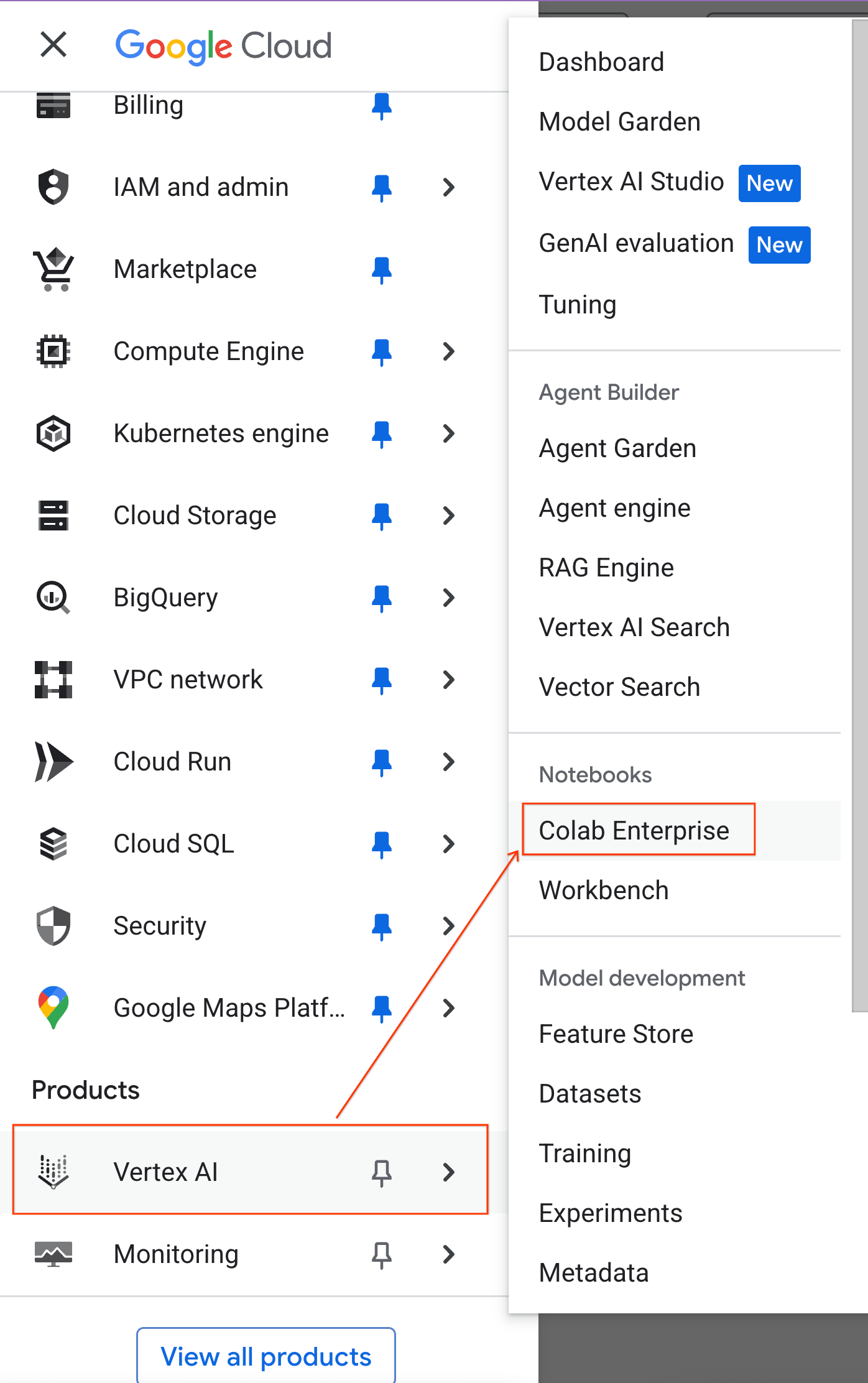
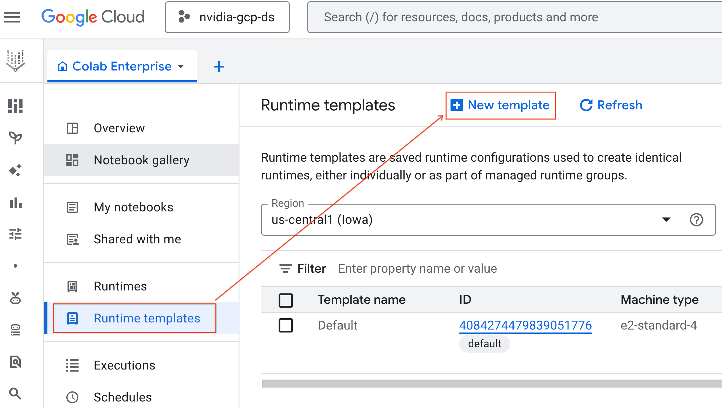
- From Colab Enterprise, click Runtime templates and then select New Template.
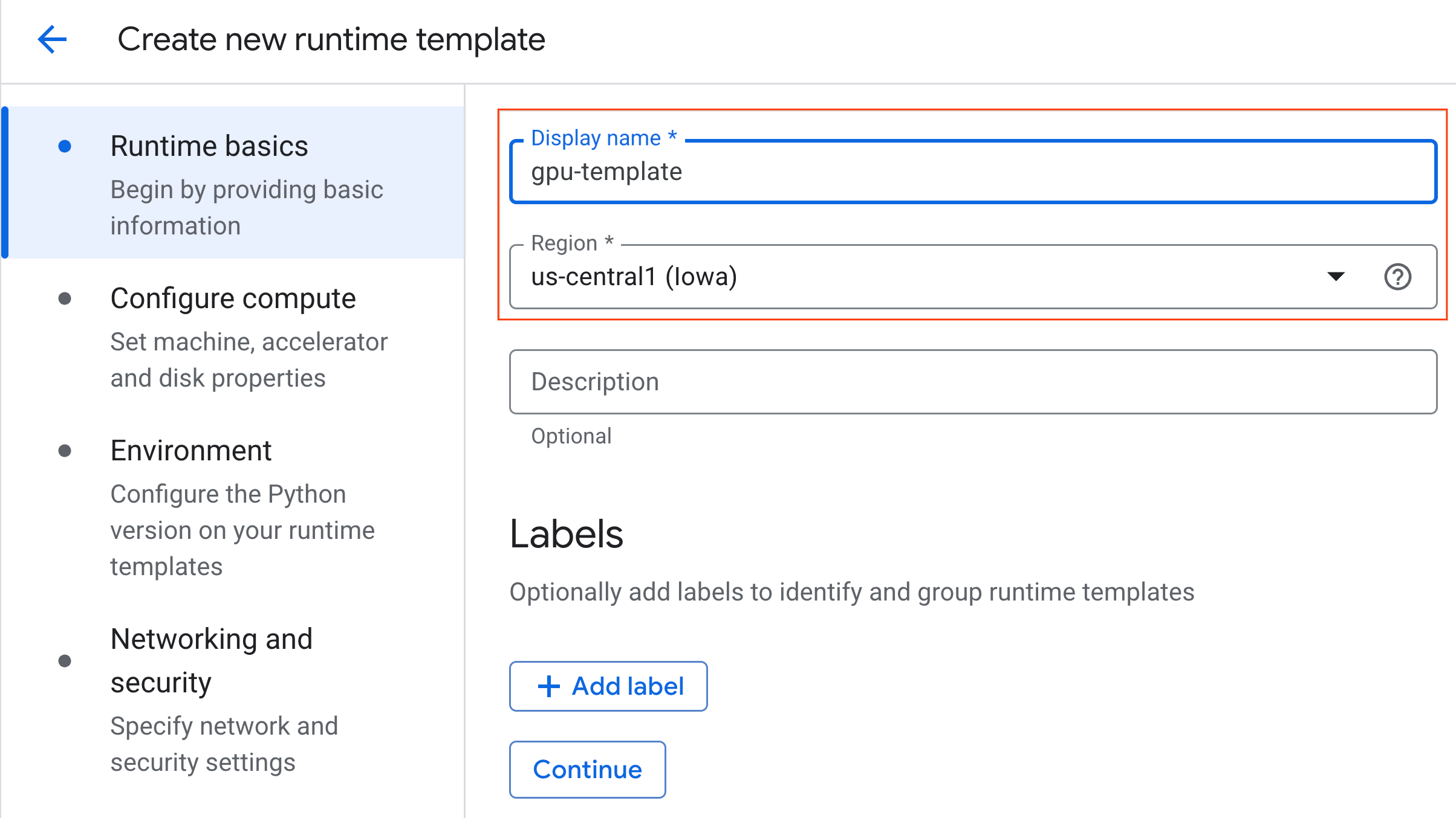
- Under Runtime basics:
- Set the Display name as
gpu-template. - Set your preferred Region.
- Set the Display name as
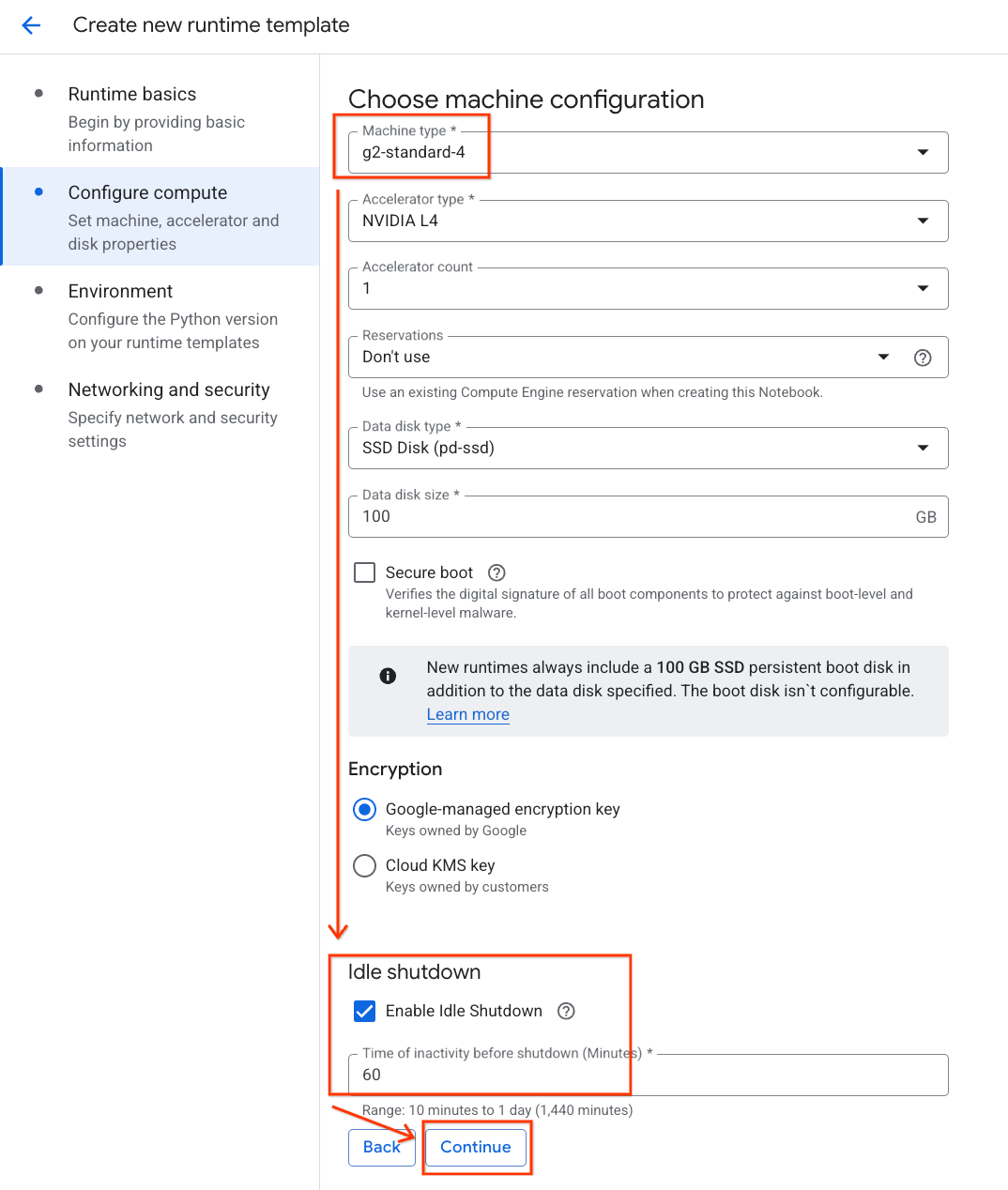
- Under Configure compute:
- Set the Machine type to
g2-standard-4. - Keep the default Accelerator Type as
NVIDIA L4with an Accelerator count of 1. - Change the Idle shutdown to 60 minutes.
- Click Continue.
- Set the Machine type to
- Under Environment:
- Set the Environment to
Python 3.11
- Set the Environment to
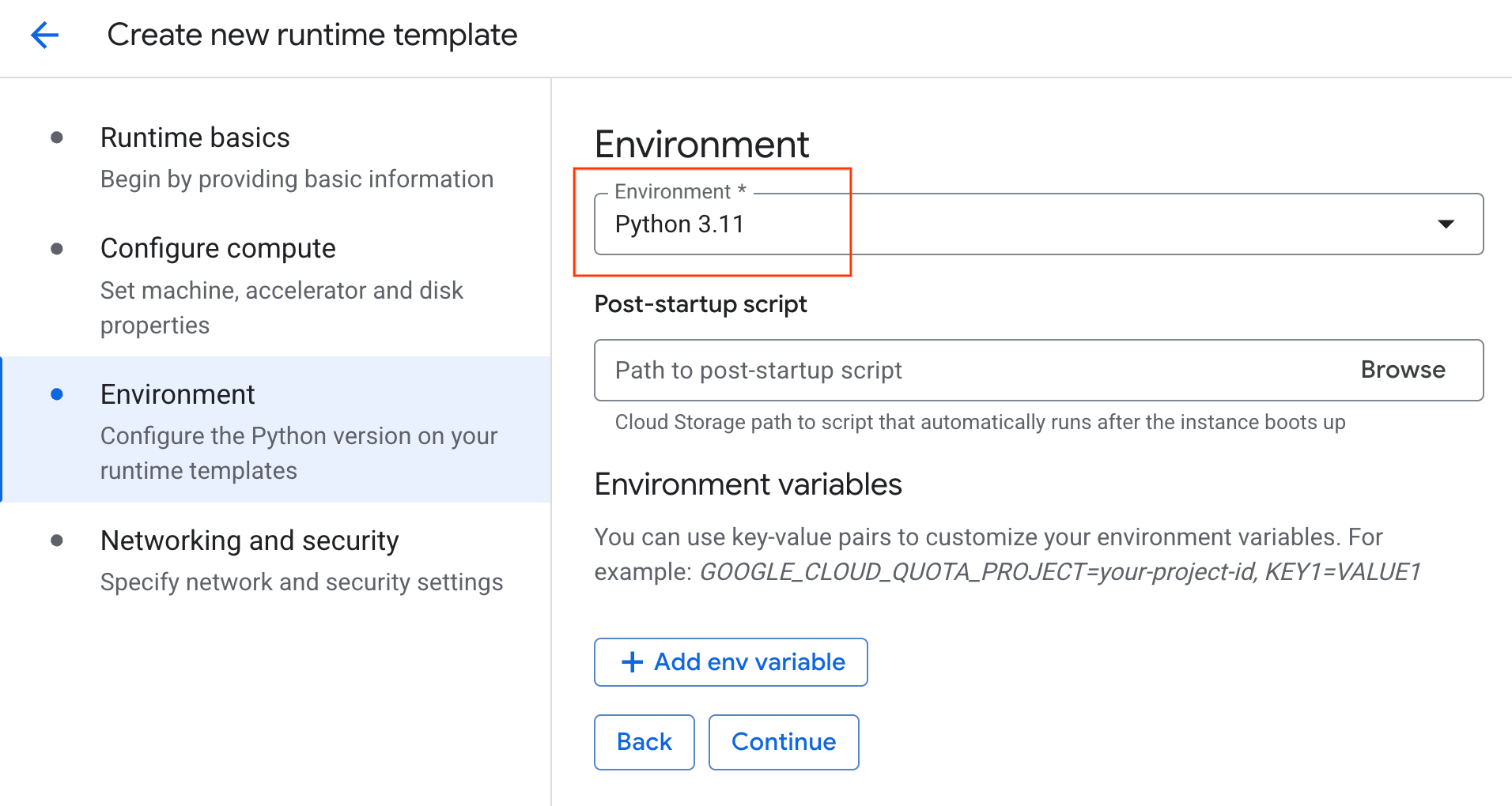
- Click Create to save the runtime template. Your Runtime templates page should now display the new template.
5. Start a runtime
With your template ready, you can create a new runtime.
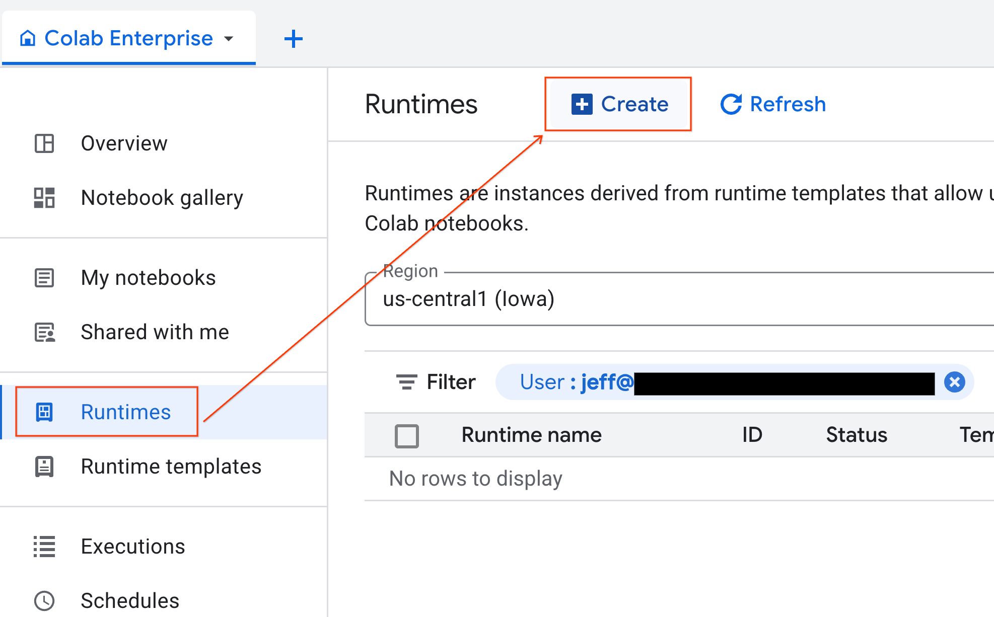
- From Colab Enterprise, click Runtimes and then select Create.
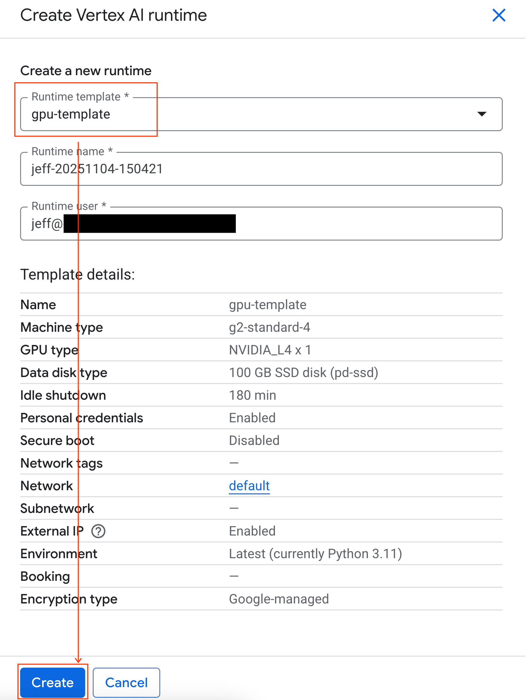
- Under Runtime template, select the
gpu-templateoption. Click Create and wait for the runtime to boot up.
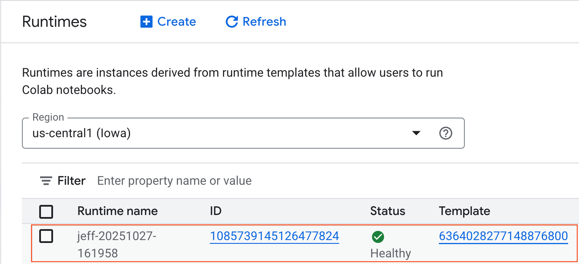
- After a few minutes, you will see the runtime available.
6. Set up the notebook
Now that your infrastructure is running, you need to import the lab notebook and connect it to your runtime.
Import the notebook
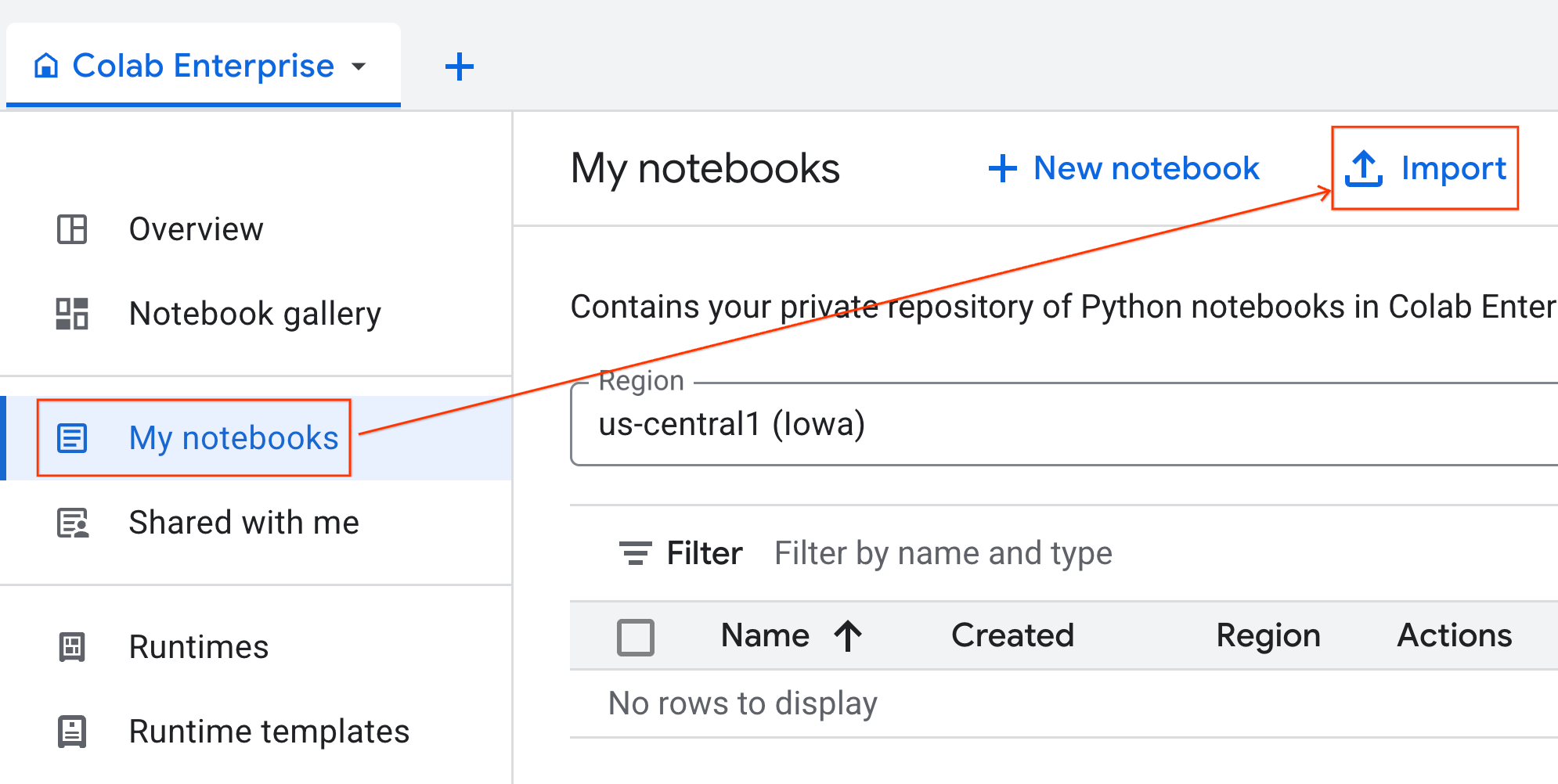
- From Colab Enterprise, click My notebooks and then click Import.
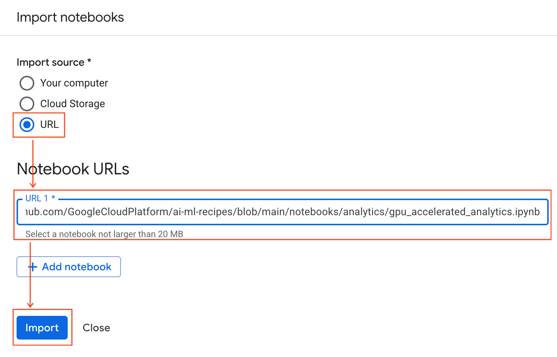
- Select the URL radio button and input the following URL:
https://github.com/GoogleCloudPlatform/ai-ml-recipes/blob/main/notebooks/analytics/gpu_accelerated_analytics.ipynb
- Click Import. Colab Enterprise will copy the notebook from GitHub into your environment.
Connect to the runtime
- Open the newly imported notebook.
- Click the down arrow next to Connect.
- Select Connect to a Runtime.
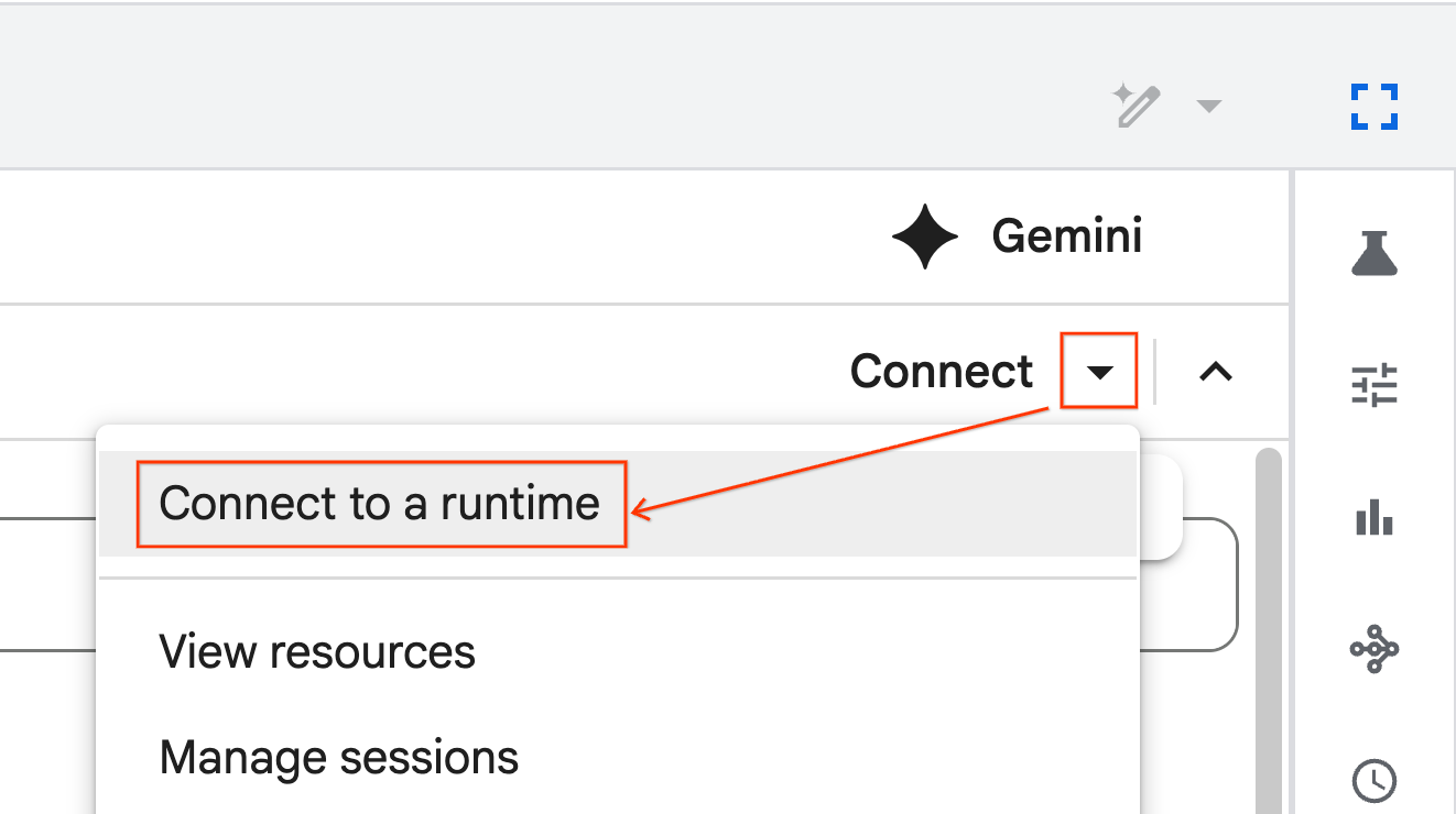
- Use the dropdown and select the runtime you previously created.
- Click Connect.
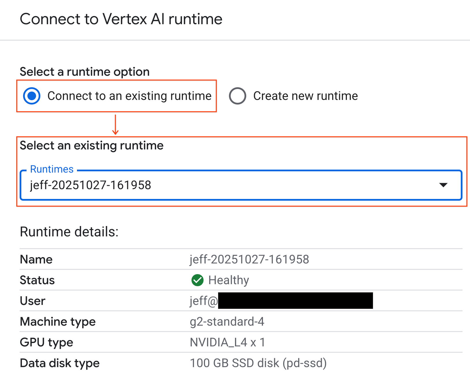
Your notebook is now connected to a GPU-enabled runtime. Now you can begin running queries!
7. Prepare the NYC taxi dataset
This Codelab uses the NYC Taxi & Limousine Commission (TLC) Trip Record Data.
The dataset contains individual trip records from yellow taxis in New York City, and includes fields like:
- Pick-up and drop-off dates, times, and locations
- Trip distances
- Itemized fare amounts
- Passenger counts
Download the data
Next, download the trip data for all of 2024. The data is stored in the Parquet file format.
The following code block performs these steps:
- Defines the range of years and months to download.
- Creates a local directory named
nyc_taxi_datato store the files. - Loops through each month, downloads the corresponding Parquet file if it doesn't already exist, and saves it to the directory.
Run this code in your notebook to gather the data and store it on the runtime:
from tqdm import tqdm
import requests
import time
import os

YEAR = 2024
DATA_DIR = "nyc_taxi_data"

os.makedirs(DATA_DIR, exist_ok=True)
print(f"Checking/Downloading files for {YEAR}...")


for month in tqdm(range(1, 13), unit="file"):

    # Define standardized filename for both local path and URL
    file_name = f"yellow_tripdata_{YEAR}-{month:02d}.parquet"
    local_path = os.path.join(DATA_DIR, file_name)
    url = f"https://d37ci6vzurychx.cloudfront.net/trip-data/{file_name}"

    if not os.path.exists(local_path):
        try:
            with requests.get(url, stream=True) as response:
                response.raise_for_status()
                with open(local_path, 'wb') as f:
                    for chunk in response.iter_content(chunk_size=8192):
                        f.write(chunk)
            time.sleep(1)
        except requests.exceptions.HTTPError as e:

            print(f"\nSkipping {file_name}: {e}")

            if os.path.exists(local_path):
                os.remove(local_path)

print("\nDownload complete.")
8. Explore the taxi trip data
Now that you've downloaded the dataset, it's time to perform an initial exploratory data analysis (EDA). The goal of EDA is to understand the data's structure, find anomalies, and uncover potential patterns.
Load a single month of data
Begin by loading a single month's worth of data. This provides a large enough sample (over 3 million rows) to be meaningful while keeping memory usage manageable for interactive analysis.
import pandas as pd
import glob

# Load the last month of the downloaded data
df = pd.read_parquet("nyc_taxi_data/yellow_tripdata_2024-12.parquet")
df.head()
Get summary statistics
Use the .describe() method to generate high-level summary statistics for the numerical columns. This is a great first step to spot potential data quality issues, such as unexpected minimum or maximum values.
df.describe().round(2)
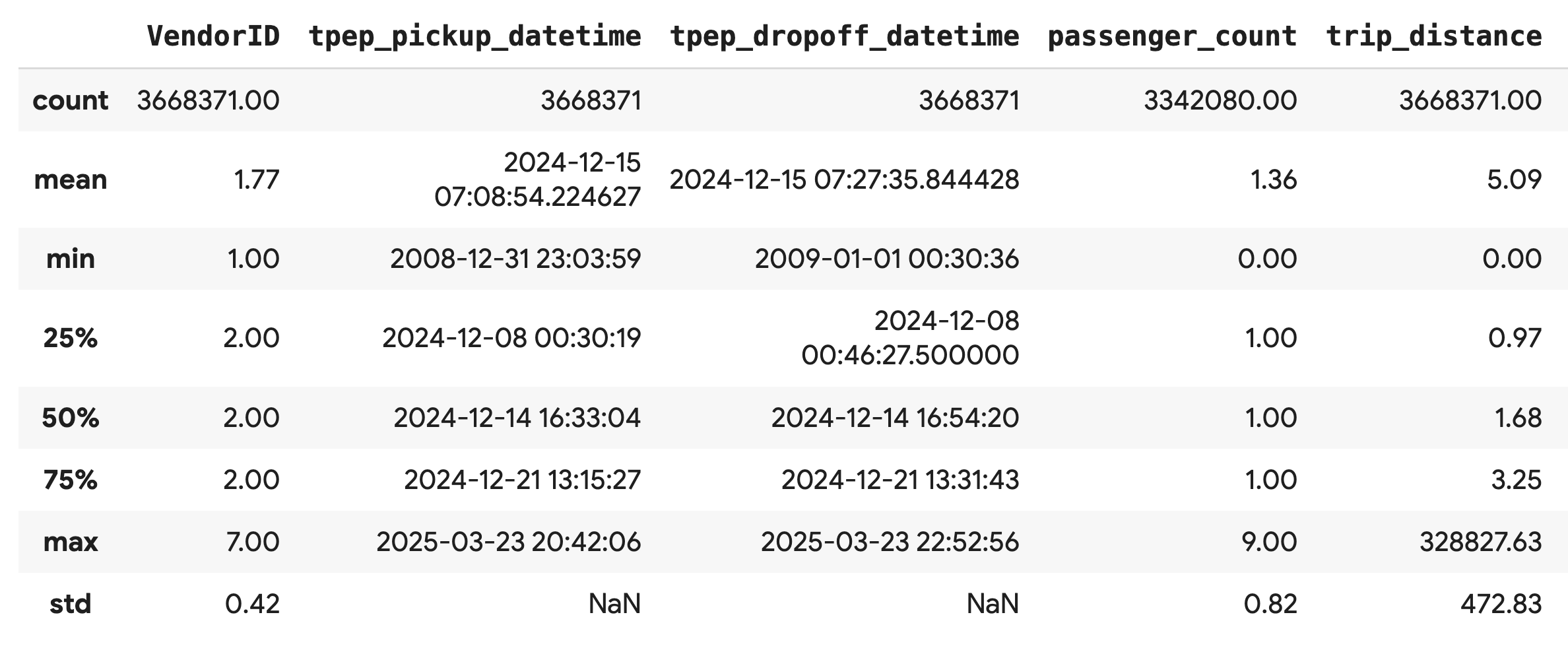
Investigate data quality
The output from .describe() immediately reveals an issue. Notice that the min value for tpep_pickup_datetime and tpep_dropoff_datetime is in the year 2008, which doesn't make sense for a 2024 dataset.
This is an example of why to always inspect your data. You can investigate this further by sorting the DataFrame to find the exact rows that contain these outlier dates.
# Sort by the dropoff datetime to see the oldest records
df.sort_values("tpep_pickup_datetime").head()
Visualize data distributions
Next, you can create histograms of the numerical columns to visualize their distributions. This helps you understand the spread and skew of features like trip_distance and fare_amount. The .hist() function is a quick way to plot histograms for all numerical columns in a DataFrame.
_ = df.hist(figsize=(20, 20))
Finally, generate a scatter matrix to visualize the relationships between a few key columns. Because plotting millions of points is slow and can obscure patterns, use .sample() to create the plot from a random sample of 100,000 rows.
_ = pd.plotting.scatter_matrix(
    df[['passenger_count', 'trip_distance', 'tip_amount', 'total_amount']].sample(100_000),
    diagonal="kde",
    figsize=(15, 15)
)
9. Why use the Parquet file format?
The NYC taxi dataset is provided in Apache Parquet format. This is a deliberate choice made for large-scale analytics. Parquet offers several advantages over file types like CSV:
- Efficient and Fast: As a columnar format, Parquet is highly efficient to store and read. It supports modern compression methods that result in smaller file sizes and significantly faster I/O, especially on GPUs.
- Preserves the Schema: Parquet stores data types in the file's metadata. You never have to guess data types when you read the file.
- Enables Selective Reading: The columnar structure allows you to read only the specific columns you need for an analysis. This can dramatically reduce the amount of data you have to load into memory.
Explore Parquet features
Let's explore two of these powerful features using one of the files you downloaded.
Inspect metadata without loading the full dataset
While you can't view a Parquet file in a standard text editor, you can easily inspect its schema and metadata without loading any data into memory. This is useful for quickly understanding the structure of a file.
from pyarrow.parquet import ParquetFile
import pyarrow as pa

# Open one of the downloaded files
pf = ParquetFile('nyc_taxi_data/yellow_tripdata_2024-12.parquet')

# Print the schema
print("File Schema:")
print(pf.schema)

# Print the file metadata
print("\nFile Metadata:")
print(pf.metadata)
Read only the columns you need
Imagine you only need to analyze trip distance and fare amounts. With Parquet, you can load just those columns, which is much faster and more memory-efficient than loading the entire DataFrame.
import pandas as pd

# Read only four specific columns from the Parquet file
df_subset = pd.read_parquet(
    'nyc_taxi_data/yellow_tripdata_2024-12.parquet',
    columns=['passenger_count', 'trip_distance', 'tip_amount', 'total_amount']
)

df_subset.head()
10. Accelerate pandas with NVIDIA cuDF
NVIDIA CUDA for DataFrames (cuDF) is an open-source, GPU-accelerated library that allows you to interact with DataFrames. cuDF lets you to perform common data operations like filtering, joining, and grouping on the GPU with massive parallelism.
The key feature you use in this Codelab is the cudf.pandas accelerator mode. When you enable it, your standard pandas code is automatically redirected to use GPU-powered cuDF kernels under the hood, all without requiring you to change your code.
Enable GPU acceleration
To use NVIDIA cuDF in a Colab Enterprise notebook, you load its magic extension before you import pandas.
First, inspect the standard pandas library. Notice the output shows the path to the default pandas installation.
import pandas as pd
pd # Note the output for the standard pandas library
Now, load the cudf.pandas extension and import pandas again. Watch how the output for the pd module changes - this confirms that the GPU-accelerated version is now active.
%load_ext cudf.pandas
import pandas as pd
pd # Note the new output, indicating cudf.pandas is active
Other ways to enable cudf.pandas
While the magic command (%load_ext) is the easiest method in a notebook, you can also enable the accelerator in other environments:
- In Python scripts: Call
import cudf.pandasandcudf.pandas.install()before yourpandasimport. - From non-notebook environments: Run your script using
python -m cudf.pandas your_script.py.
11. Compare CPU vs. GPU performance
Now for the most important part: comparing the performance of standard pandas on a CPU with cudf.pandas on a GPU.
To ensure a completely fair baseline for the CPU, you must first reset the Colab runtime. This clears any GPU accelerators you might have enabled in the previous sections. You can restart runtime by running the following cell, or selecting Restart session from the Runtime menu.
import IPython

IPython.Application.instance().kernel.do_shutdown(True)
Define the analytics pipeline
Now that the environment is clean, you will define the benchmarking function. This function allows you to run the exact same pipeline - loading, sorting, and summarizing - using whichever pandas module you pass to it.
import time
import glob
import numpy as np
import pandas as pd
import matplotlib.pyplot as plt

def run_analytics_pipeline(pd_module):
    """Loads, sorts, and summarizes data using the provided pandas module."""
    timings = {}

    # 1. Load all 2024 Parquet files from the directory
    t0 = time.time()
    df = pd_module.concat(
        [pd_module.read_parquet(f) for f in glob.glob("nyc_taxi_data/*_2024*.parquet")],
        ignore_index=True
    )
    timings["load"] = time.time() - t0

    # 2. Sort the data by multiple columns
    t0 = time.time()
    df = df.sort_values(
        ['tpep_pickup_datetime', 'trip_distance', 'passenger_count'],
        ascending=[False, True, False]
    )
    timings["sort"] = time.time() - t0

    # 3. Perform a groupby and aggregation
    t0 = time.time()
    df['tpep_pickup_datetime'] = pd_module.to_datetime(df['tpep_pickup_datetime'])
    _ = (
        df.loc[df.tpep_pickup_datetime > '2024-11-01']
          .groupby(['VendorID', 'tpep_pickup_datetime'])
          [['passenger_count', 'fare_amount']]
          .agg(['min', 'mean', 'max'])
    )
    timings["summarize"] = time.time() - t0

    return timings
Run the comparison
First, you will run the pipeline using standard pandas on the CPU. Then, you enable cudf.pandas and run it again on the GPU.
# --- Run on CPU ---
print("Running analytics pipeline on CPU...")
# Ensure we are using standard pandas
import pandas as pd
assert "cudf" not in str(pd), "Error: cuDF is still active. Please restart the kernel."

cpu_times = run_analytics_pipeline(pd)
print(f"CPU times: {cpu_times}")

# --- Run on GPU ---
print("\nEnabling cudf.pandas and running on GPU...")
# Load the extension
%load_ext cudf.pandas
import pandas as gpu_pd

gpu_times = run_analytics_pipeline(gpu_pd)
print(f"GPU times: {gpu_times}")
Visualize the results
Finally, visualize the difference. The following code calculates the speedup for each operation and plots them side-by-side.
# Create a DataFrame for plotting
results_df = pd.DataFrame([cpu_times, gpu_times], index=["CPU", "GPU"]).T
total_cpu_time = results_df['CPU'].sum()
total_gpu_time = results_df['GPU'].sum()
speedup = total_cpu_time / total_gpu_time

print("--- Performance Results ---")
print(results_df)
print(f"\nTotal CPU Time: {total_cpu_time:.2f} seconds")
print(f"Total GPU Time: {total_gpu_time:.2f} seconds")
print(f"Overall Speedup: {speedup:.2f}x")

# Plot the results
fig, ax = plt.subplots(figsize=(10, 6))
results_df.plot(kind='bar', ax=ax, color={"CPU": "tab:blue", "GPU": "tab:green"})

ax.set_ylabel("Time (seconds)")
ax.set_title(f"CPU vs. GPU Runtimes (Overall Speedup: {speedup:.2f}x)", fontsize=14)
ax.tick_params(axis='x', rotation=0)

# Add numerical labels to the bars
for container in ax.containers:
    ax.bar_label(container, fmt="%.2f", padding=3)

plt.tight_layout()
plt.show()
Sample results:
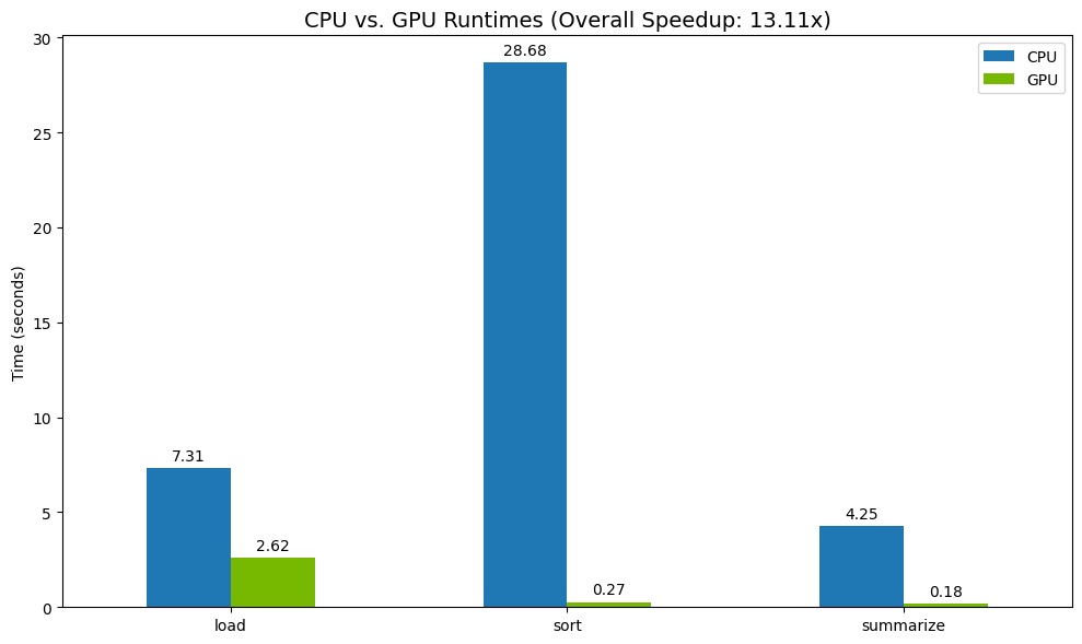
The GPU provides a clear speed increase relative to the CPU.
12. Profile your code to find bottlenecks
Even with GPU acceleration, some pandas operations might fall back to the CPU if they are not yet supported by cuDF. These "CPU fallbacks" can become performance bottlenecks.
To help you identify these areas, cudf.pandas includes two built-in profilers. You can use them to see exactly which parts of your code are running on the GPU and which are falling back to the CPU.
%%cudf.pandas.profile: Use this for a high-level, function-by-function summary of your code. It's best for getting a quick overview of which operations are running on which device.%%cudf.pandas.line_profile: Use this for a detailed, line-by-line analysis. It's the best tool for pinpointing the exact lines in your code that are causing a fallback to the CPU.
Use these profilers as "cell magics" at the top of a notebook cell.
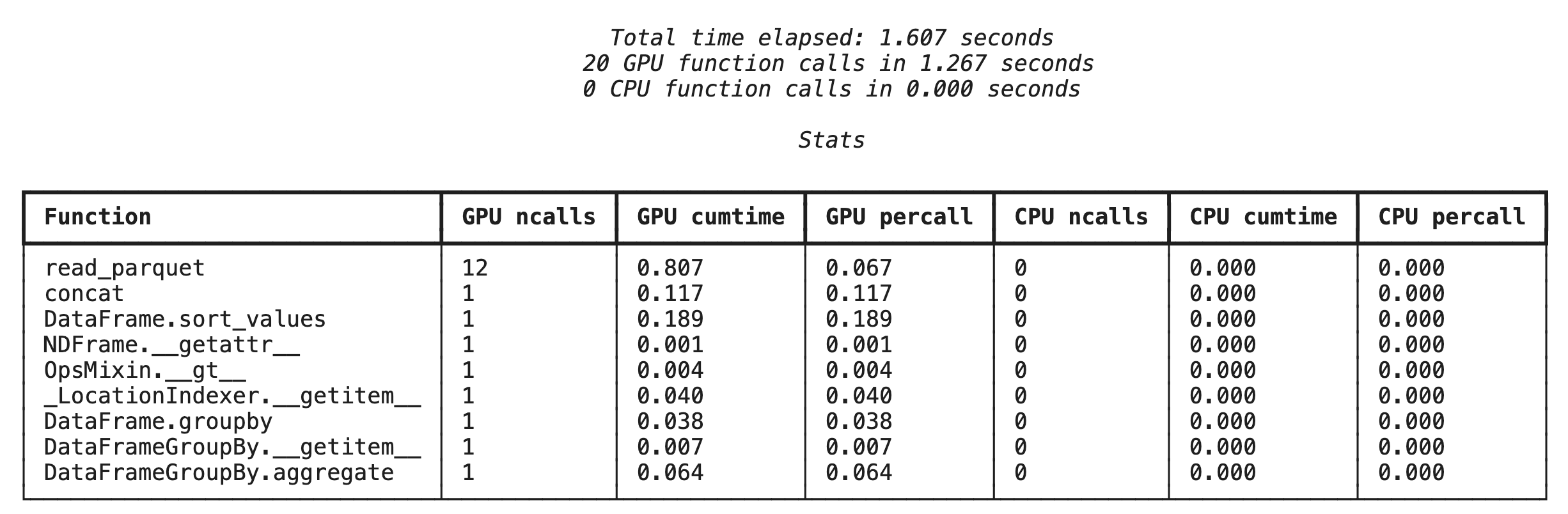
Function-level profiling with %%cudf.pandas.profile
First, run the function-level profiler on the same analytics pipeline from the previous section. The output shows a table of every function called, the device it ran on (GPU or CPU), and how many times it was called.
%load_ext cudf.pandas
import pandas as pd
import glob

pd.DataFrame({"a": [1]})
After ensuring cudf.pandas is active, you can run a profile.
%%cudf.pandas.profile

df = pd.concat([pd.read_parquet(f) for f in glob.glob("nyc_taxi_data/*2024*.parquet")], ignore_index=True)

df = df.sort_values(['tpep_pickup_datetime', 'trip_distance', 'passenger_count'], ascending=[False, True, False])

summary = (
    df
        .loc[(df.tpep_pickup_datetime > '2024-11-01')]
        .groupby(['VendorID','tpep_pickup_datetime'])
        [['passenger_count', 'fare_amount']]
        .agg(['min', 'mean', 'max'])
)
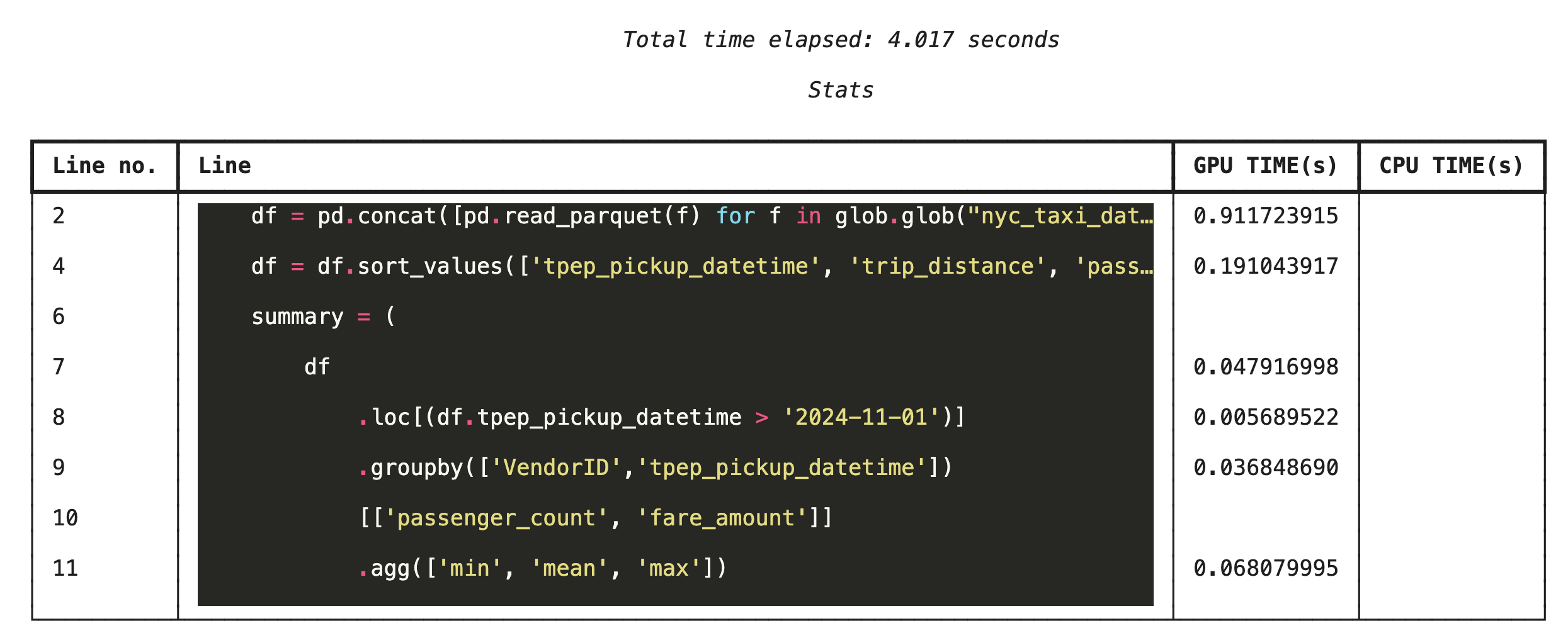
Line-by-line profiling with %%cudf.pandas.line_profile
Next, run the line-level profiler. This gives you a much more granular view, showing the portion of time each line of code spent executing on the GPU versus the CPU. This is the most effective way to find specific bottlenecks to optimize.
%%cudf.pandas.line_profile

df = pd.concat([pd.read_parquet(f) for f in glob.glob("nyc_taxi_data/*2024*.parquet")], ignore_index=True)

df = df.sort_values(['tpep_pickup_datetime', 'trip_distance', 'passenger_count'], ascending=[False, True, False])

summary = (
    df
        .loc[(df.tpep_pickup_datetime > '2024-11-01')]
        .groupby(['VendorID','tpep_pickup_datetime'])
        [['passenger_count', 'fare_amount']]
        .agg(['min', 'mean', 'max'])
)
Profiling from the command line
These profilers are also available from the command line, which is useful for automated testing and profiling of Python scripts.
You can use the following on a command line interface:
python -m cudf.pandas --profile your_script.pypython -m cudf.pandas --line_profile your_script.py
13. Integrate with Google Cloud Storage
Google Cloud Storage (GCS) is a scalable and durable object storage service. When you use Colab Enterprise, GCS is a great place to store your datasets, model checkpoints, and other artifacts.
Your Colab Enterprise runtime has the necessary permissions to read and write data directly to GCS buckets, and these operations are GPU-accelerated for maximum performance.
Create a GCS bucket
First, create a new GCS bucket. GCS bucket names are globally unique, so append a UUID to its name.
from google.cloud import storage
import uuid

unique_suffix = uuid.uuid4().hex[:12]
bucket_name = f'nyc-taxi-codelab-{unique_suffix}'
project_id = storage.Client().project

client = storage.Client()

try:
    bucket = client.create_bucket(bucket_name)
    print(f"Successfully created bucket: gs://{bucket.name}")
except Exception as e:
    print(f"Bucket creation failed. You may already own it or the name is taken: {e}")
Write data directly to GCS
Now, save a DataFrame directly to your new GCS bucket. If the df variable isn't available from the previous sections, the code first loads a single month of data.
%%cudf.pandas.line_profile

# Ensure the DataFrame exists before saving to GCS
if 'df' not in locals():
    print("DataFrame not found, loading a sample file...")
    df = pd.read_parquet('nyc_taxi_data/yellow_tripdata_2024-12.parquet')

print(f"Writing data to gs://{bucket_name}/nyc_taxi_data.parquet...")
df.to_parquet(f"gs://{bucket_name}/nyc_taxi_data.parquet", index=False)
print("Write operation complete.")
Verify the file in GCS
You can verify the data is in GCS by visiting the bucket. The following code creates a clickable link.
from IPython.display import Markdown

gcs_url = f"https://console.cloud.google.com/storage/browser/{bucket_name}?project={project_id}"
Markdown(f'**[Click here to view your GCS bucket in the Google Cloud Console]({gcs_url})**')
Read data directly from GCS
Finally, read data directly from a GCS path into a DataFrame. This operation is also GPU-accelerated, allowing you to load large datasets from cloud storage at high speed.
%%cudf.pandas.line_profile

print(f"Reading data from gs://{bucket_name}/nyc_taxi_data.parquet...")
df_from_gcs = pd.read_parquet(f"gs://{bucket_name}/nyc_taxi_data.parquet")

df_from_gcs.head()
14. Clean Up
To avoid incurring unexpected charges to your Google Cloud account, you need to clean up the resources you created.
Delete the data you downloaded:
# Permanately delete the GCS bucket
print(f"Deleting GCS bucket: gs://{bucket_name}...")
!gsutil rm -r -f gs://{bucket_name}
print("Bucket deleted.")

# Remove NYC taxi dataset on the Colab runtime
print("Deleting local 'nyc_taxi_data' directory...")
!rm -rf nyc_taxi_data
print("Local files deleted.")
Shut down your Colab runtime
- In the Google Cloud console, go to the Colab Enterprise Runtimes page.
- In the Region menu, select the region that contains your runtime.
- Select the runtime you want to delete.
- Click Delete.
- Click Confirm.
Delete your Notebook
- In the Google Cloud console, go to the Colab Enterprise My Notebooks page.
- In the Region menu, select the region that contains your notebook.
- Select the notebook you want to delete.
- Click Delete.
- Click Confirm.
15. Congratulations
Congratulations! You've successfully accelerated a pandas analytics workflow using NVIDIA cuDF on Colab Enterprise. You learned how to configure GPU-enabled runtimes, enable cudf.pandas for zero-code-change acceleration, profile code for bottlenecks, and integrate with Google Cloud Storage.