運用 Google Cloud 和 NVIDIA 加速資料分析

1. 簡介

在本程式碼研究室中，您將瞭解如何使用 Google Cloud 上的 NVIDIA GPU 和開放原始碼程式庫，加速處理大型資料集的資料分析工作流程。首先，您將最佳化基礎架構，然後探索如何套用 GPU 加速，完全不必變更程式碼。

您將著重於 pandas 這個熱門的資料操作程式庫，並瞭解如何使用 NVIDIA 的 cuDF 程式庫加速運算。最棒的是，您不必變更現有的 pandas 程式碼，就能取得這項 GPU 加速功能。

課程內容

• 瞭解 Google Cloud 上的 Colab Enterprise。
• 使用特定 GPU、CPU 和記憶體設定，自訂 Colab 執行階段環境。
• 使用 NVIDIA cuDF 加速 pandas，完全不必修改程式碼。
• 剖析程式碼，找出並改善效能瓶頸。

2. 為什麼要加快資料處理速度？

80/20 法則：資料準備為何如此耗時

資料準備通常是分析專案中最耗時的階段。資料科學家和分析師在開始分析前，會花費大量時間清理、轉換及建構資料。

好消息是，您可以使用 cuDF，在 NVIDIA GPU 上加速執行 pandas、Apache Spark 和 Polars 等熱門開放原始碼程式庫。即使有這項加速功能，資料準備作業仍相當耗時，原因如下：

• 來源資料很少能直接用於分析：現實世界的資料通常不一致、有遺漏值，且格式設定有問題。
• 資料品質會影響模型成效：如果資料品質不佳，即使是再精密的演算法也無用武之地。
• 規模會放大問題：處理數百萬筆記錄時，看似微小的資料問題會成為重大瓶頸。

3. 選擇筆記本環境

許多資料科學家都熟悉 Colab，並將其用於個人專案，但 Colab Enterprise 專為企業設計，提供安全、協作式且整合的筆記本體驗。

在 Google Cloud 中，您有兩個主要的代管型筆記本環境可供選擇：Colab Enterprise 和 Vertex AI Workbench。請根據專案的優先順序選擇合適的選項。

何時使用 Vertex AI Workbench

如果您的重點是控管及深度自訂，請選擇 Vertex AI Workbench。如果您需要執行下列操作，這是理想的選擇：

• 管理基礎架構和機器生命週期。
• 使用自訂容器和網路設定。
• 與 MLOps 管道和自訂生命週期工具整合。

使用 Colab Enterprise 的時機

如果您的首要考量是快速設定、簡單易用和安全協作，請選擇 Colab Enterprise。這項全代管解決方案可讓團隊專注於分析，不必煩惱基礎架構。Colab Enterprise 的優勢如下：

• 開發與資料倉儲密切相關的資料科學工作流程。您可以直接在 BigQuery Studio 開啟及管理筆記本。
• 訓練機器學習模型，並與 Vertex AI 中的 MLOps 工具整合。
• 享受彈性且統一的體驗。在 BigQuery 中建立的 Colab Enterprise 筆記本可以在 Vertex AI 中開啟及執行，反之亦然。

今日實驗室

本程式碼研究室使用 Colab Enterprise 加速資料分析。

如要進一步瞭解兩者的差異，請參閱選擇合適的 Notebook 解決方案官方說明文件。

4. 設定執行階段範本

在 Colab Enterprise 中，連線至以預先設定的執行階段範本為基礎的執行階段。

執行階段範本是可重複使用的設定，可指定筆記本的整個環境，包括：

• 機器類型 (CPU、記憶體)
• 加速器 (GPU 類型和數量)
• 磁碟大小和類型
• 網路設定和安全性政策
• 自動閒置關機規則

執行階段範本的優點

• 取得一致的環境：您和隊友每次都能取得相同的即用型環境，確保工作可重複執行。
• 預設安全工作：範本會自動強制執行貴機構的安全性政策。
• 有效管理費用：範本中預先設定了 GPU 和 CPU 等資源的大小，有助於避免意外超出預算。

建立執行階段範本

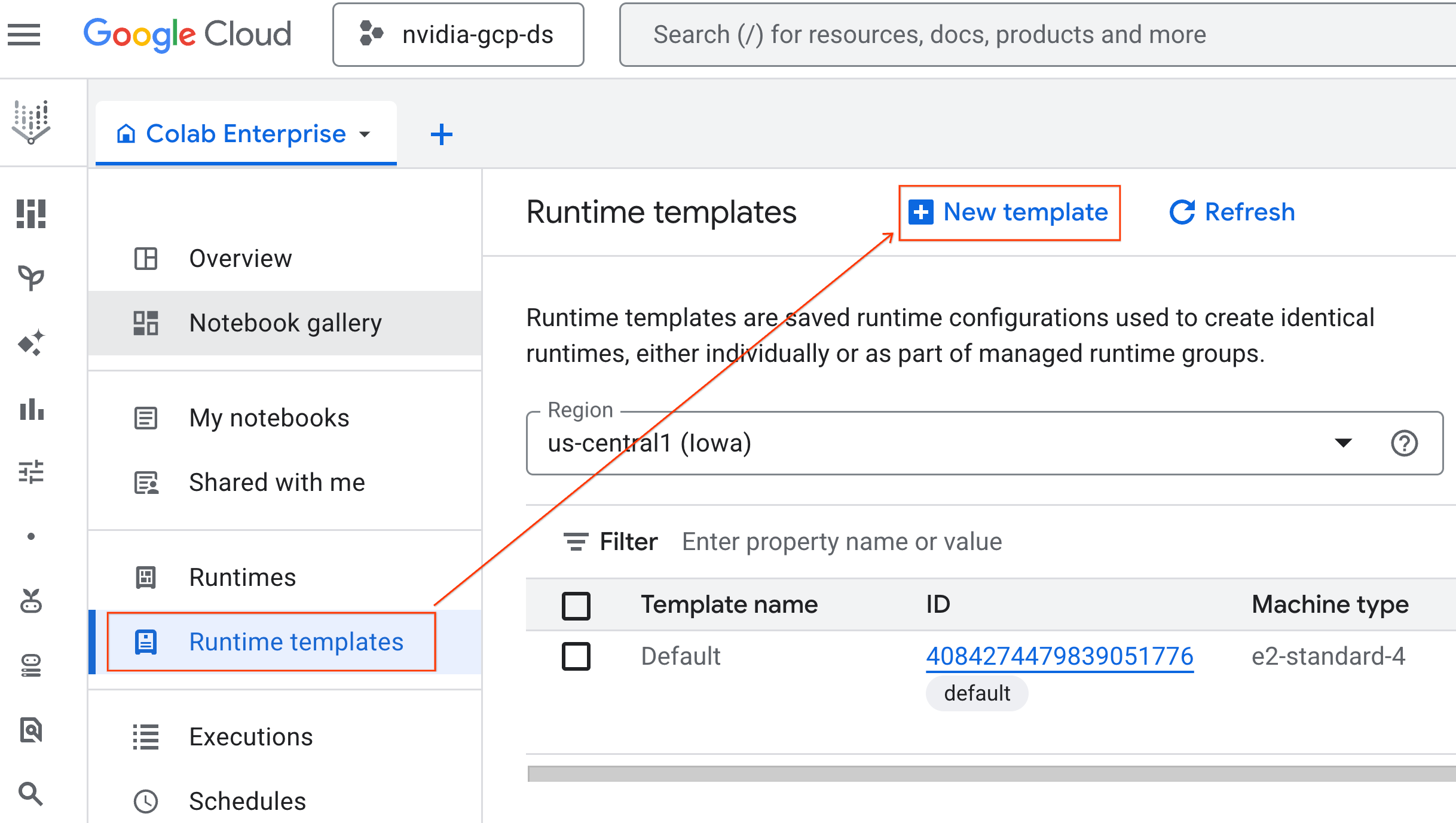
為實驗室設定可重複使用的執行階段範本。

1. 前往 Google Cloud 控制台，依序點選「導覽選單」 >「Vertex AI」 >「Colab Enterprise」

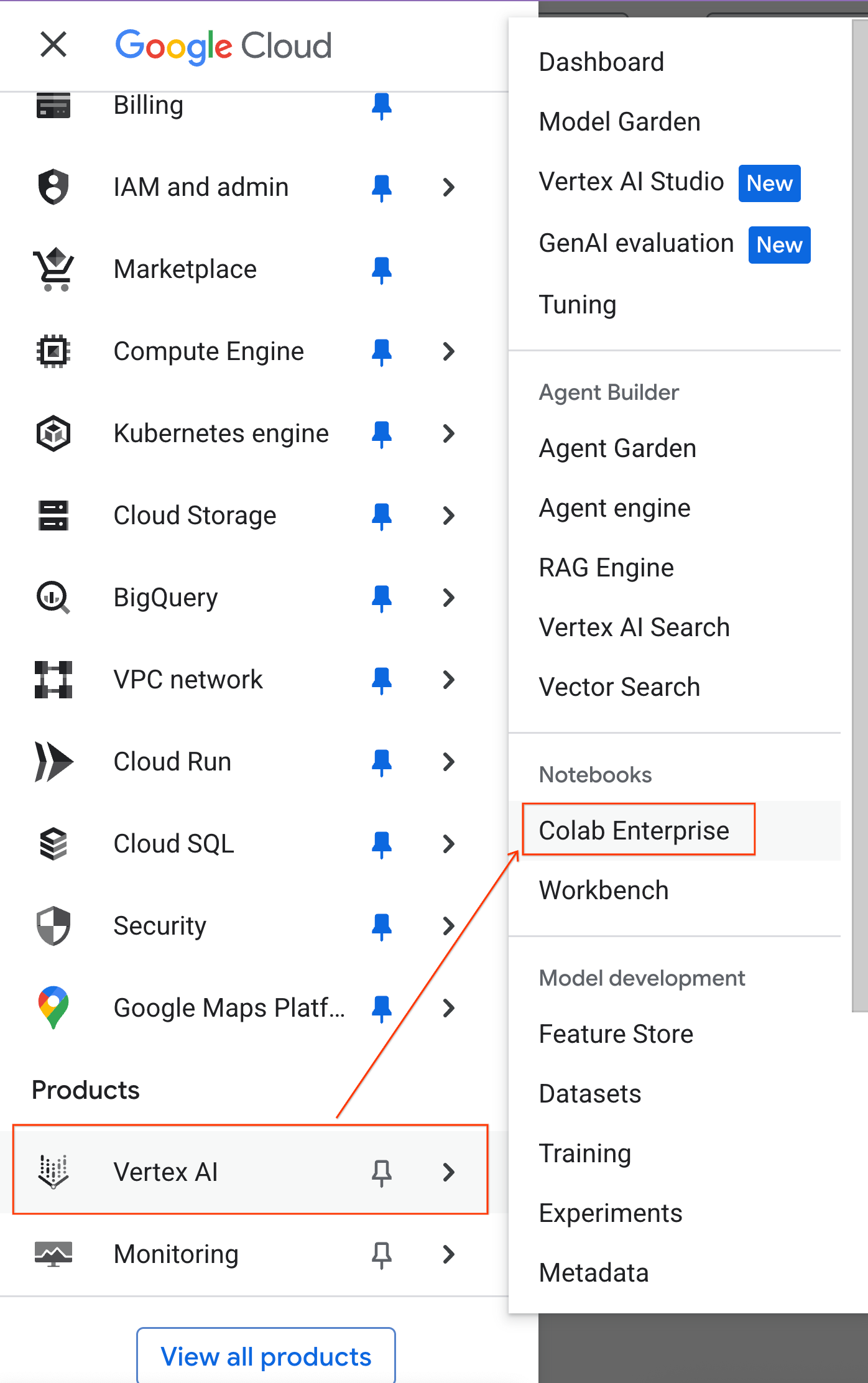
2. 在 Colab Enterprise 中，按一下「執行階段範本」，然後選取「新增範本」。

3. 在「執行階段基本資訊」下方：

• 將「Display name」(顯示名稱) 設為 gpu-template。
• 設定偏好的「地區」。

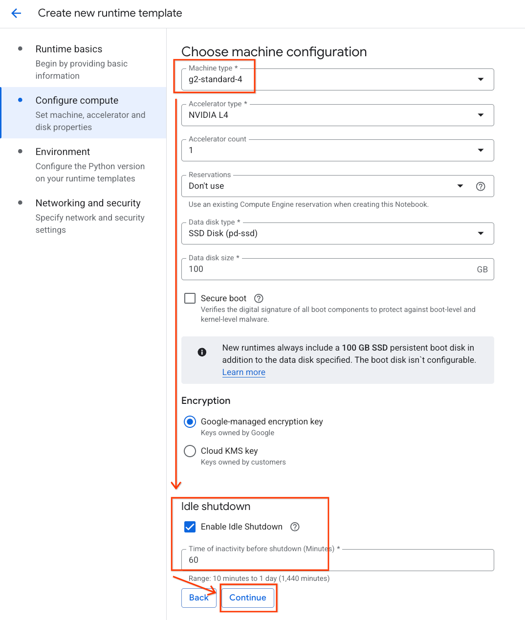
4. 在「設定運算資源」下方：

• 將「Machine type」(機器類型) 設為 g2-standard-4。
• 將「閒置關機」變更為 60 分鐘。

5. 按一下「建立」即可儲存執行階段範本。「執行階段範本」頁面現在應該會顯示新範本。

5. 啟動執行階段

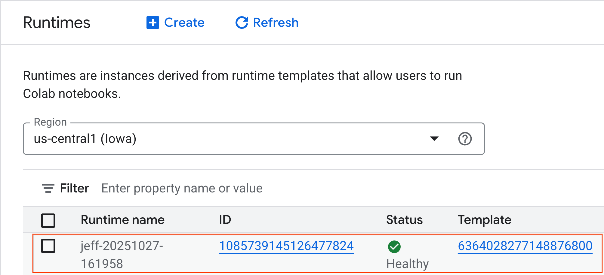
範本準備就緒後，即可建立新的執行階段。

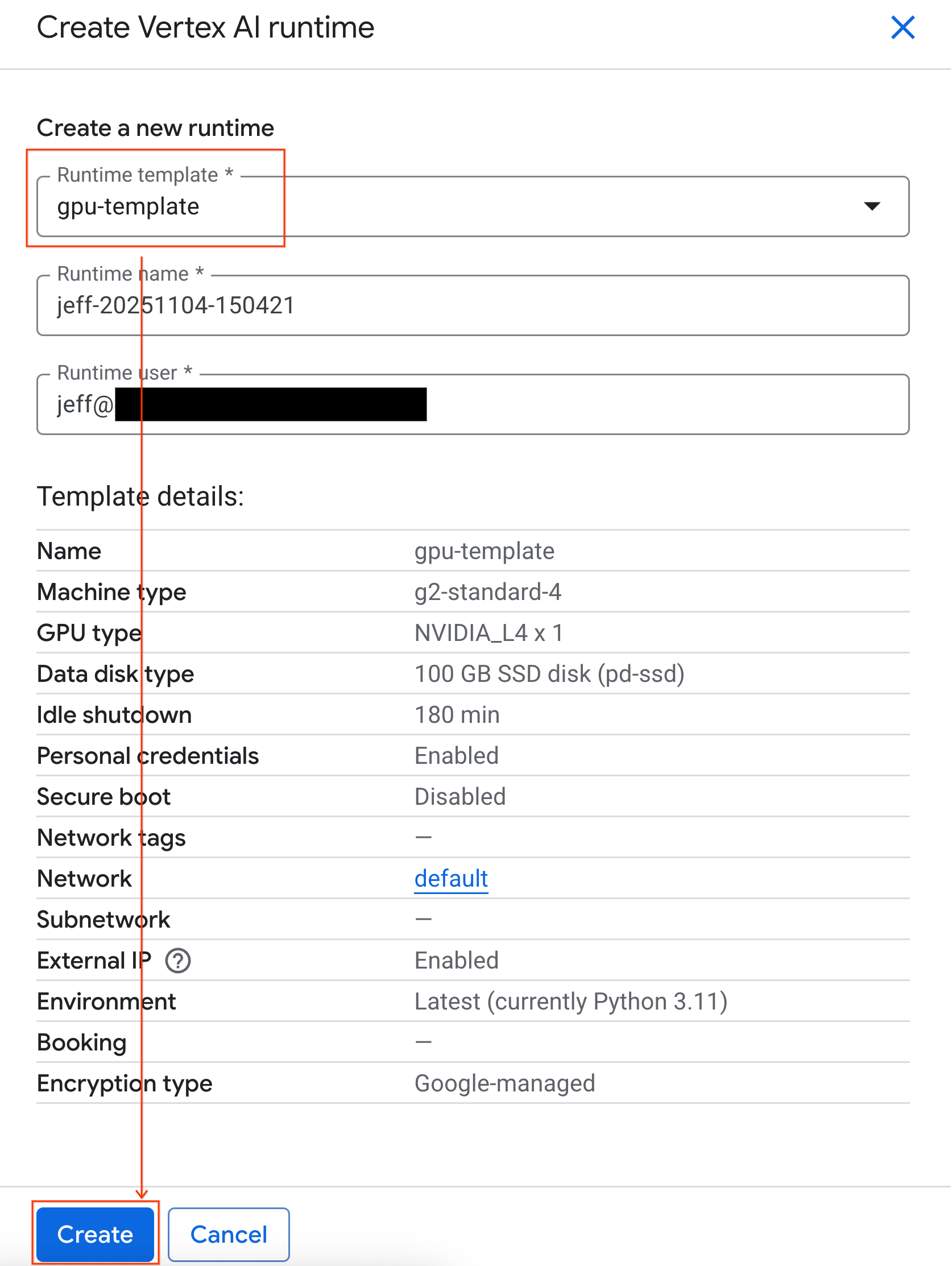
1. 在 Colab Enterprise 中，依序點選「執行階段」和「建立」。

2. 在「執行階段範本」下方，選取 gpu-template 選項。按一下「建立」，然後等待執行階段啟動。

3. 幾分鐘後，您就會看到可用的執行階段。

注意：如果收到失敗通知，請稍後幾分鐘或改用其他區域再試一次。失敗原因可能是 GPU 需求量過高。

6. 設定筆記本

基礎架構執行完畢後，您需要匯入實驗室筆記本，並將其連線至執行階段。

匯入筆記本

1. 在 Colab Enterprise 中，依序點選「我的筆記本」和「匯入」。

2. 選取「網址」圓形按鈕，然後輸入下列網址：

https://github.com/GoogleCloudPlatform/ai-ml-recipes/blob/main/notebooks/analytics/gpu_accelerated_analytics.ipynb

3. 按一下 [匯入]。Colab Enterprise 會將筆記本從 GitHub 複製到您的環境。

連線至執行階段

1. 開啟新匯入的筆記本。
2. 按一下「連結」旁的向下箭頭。
3. 選取「連線到執行階段」。

4. 使用下拉式選單，選取先前建立的執行階段。
5. 按一下「連結」。

筆記本現在已連線至啟用 GPU 的執行階段。現在可以開始執行查詢了！

注意：後續章節中的程式碼片段僅供說明用途。筆記本包含所有必要程式碼，您不需要從程式碼研究室複製及貼上程式碼。

7. 準備紐約市計程車資料集

本程式碼研究室使用紐約市計程車暨禮車管理局 (TLC) 的載客記錄資料。

這個資料集包含紐約市黃色計程車的個別行程記錄，以及下列欄位：

• 取車和還車日期、時間和地點
• 行程距離
• 車資明細金額
• 乘客人數

下載資料

接著，下載 2024 年全年的行程資料。資料會以 Parquet 檔案格式儲存。

下列程式碼區塊會執行這些步驟：

1. 定義要下載的年份和月份範圍。
2. 建立名為 nyc_taxi_data 的本機目錄，用於儲存檔案。
3. 逐月循環，下載對應的 Parquet 檔案 (如果檔案尚不存在)，並儲存至目錄。

在筆記本中執行這段程式碼，即可收集資料並儲存在執行階段：

from tqdm import tqdm
import requests
import time
import os

YEAR = 2024
DATA_DIR = "nyc_taxi_data"

os.makedirs(DATA_DIR, exist_ok=True)
print(f"Checking/Downloading files for {YEAR}...")


for month in tqdm(range(1, 13), unit="file"):
    
    # Define standardized filename for both local path and URL
    file_name = f"yellow_tripdata_{YEAR}-{month:02d}.parquet"
    local_path = os.path.join(DATA_DIR, file_name)
    url = f"https://d37ci6vzurychx.cloudfront.net/trip-data/{file_name}"

    if not os.path.exists(local_path):
        try:
            with requests.get(url, stream=True) as response:
                response.raise_for_status()
                with open(local_path, 'wb') as f:
                    for chunk in response.iter_content(chunk_size=8192):
                        f.write(chunk)
            time.sleep(1)
        except requests.exceptions.HTTPError as e:

            print(f"\nSkipping {file_name}: {e}")

            if os.path.exists(local_path):
                os.remove(local_path)

print("\nDownload complete.")

8. 探索計程車行程資料

下載資料集後，現在可以執行初步的探索性資料分析 (EDA)。EDA 的目標是瞭解資料結構、找出異常狀況，以及發掘潛在模式。

載入單月資料

首先載入一個月的資料。這可提供足夠大的樣本 (超過 300 萬列)，確保分析結果有意義，同時讓記憶體用量維持在可管理的範圍內，方便進行互動式分析。

import pandas as pd
import glob

# Load the last month of the downloaded data
df = pd.read_parquet("nyc_taxi_data/yellow_tripdata_2024-12.parquet")
df.head()

取得摘要統計資料

使用 .describe() 方法，為數值資料欄產生高階摘要統計資料。這是找出潛在資料品質問題 (例如非預期的最小值或最大值) 的絕佳第一步。

df.describe().round(2)

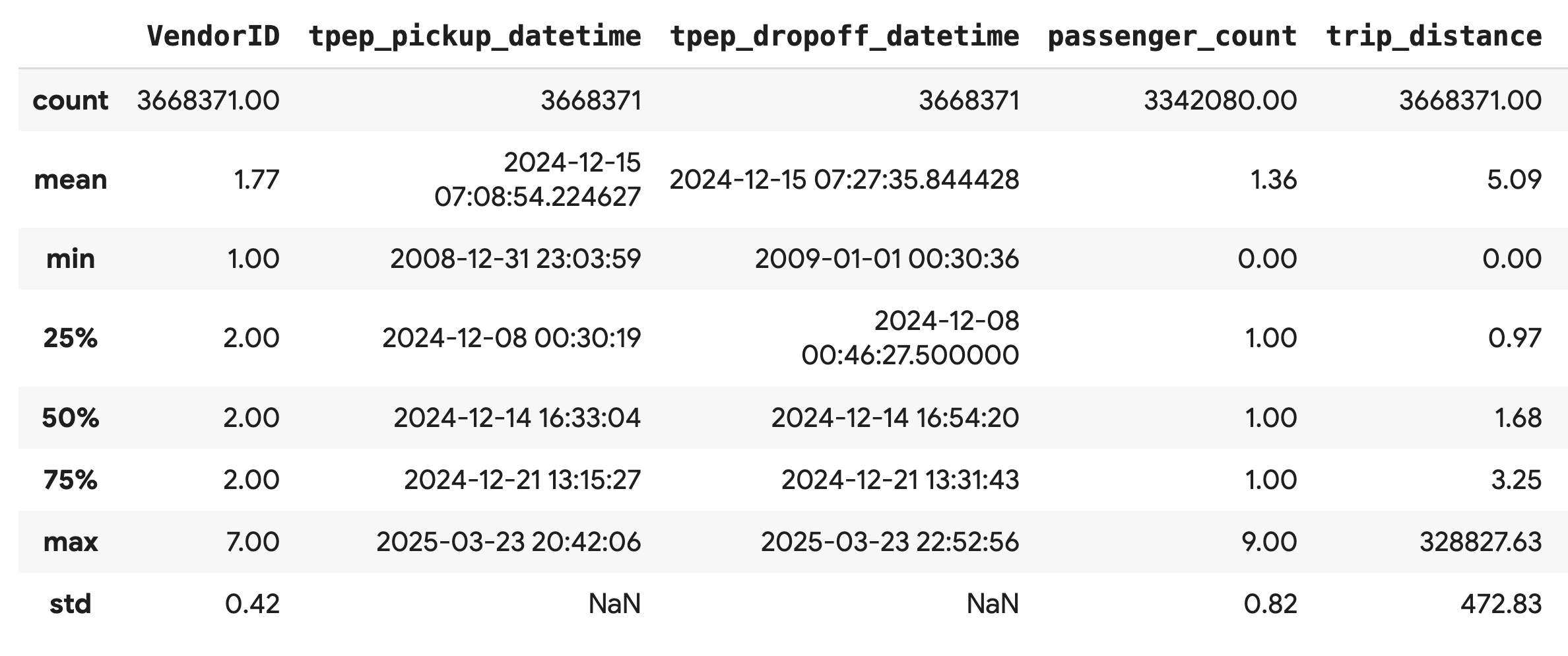
調查資料品質

.describe() 的輸出內容會立即顯示問題。請注意，tpep_pickup_datetime 和 tpep_dropoff_datetime 的 min 值為 2008 年，這對 2024 年的資料集來說並不合理。

這個例子說明瞭為什麼要一律檢查資料。您可以進一步調查，方法是排序 DataFrame，找出包含這些離群值的確切資料列。

# Sort by the dropoff datetime to see the oldest records
df.sort_values("tpep_pickup_datetime").head()

以視覺化方式呈現資料分布

接著，您可以建立數值資料欄的直方圖，以視覺化方式呈現資料分布情形。這有助於瞭解 trip_distance 和 fare_amount 等特徵的分布和偏斜情形。.hist() 函式可快速繪製 DataFrame 中所有數值資料欄的直方圖。

_ = df.hist(figsize=(20, 20))

最後，產生散布矩陣，以視覺化方式呈現幾個重要資料欄之間的關係。由於繪製數百萬個點的速度緩慢，且可能會遮蓋模式，因此請使用 .sample() 從 100,000 列的隨機樣本建立繪圖。

_ = pd.plotting.scatter_matrix(
    df[['passenger_count', 'trip_distance', 'tip_amount', 'total_amount']].sample(100_000),
    diagonal="kde",
    figsize=(15, 15)
)

注意：本程式碼研究室使用 NVIDIA GPU 加速記憶體內 pandas。如果資料已儲存在 BigQuery 中，且您要進行大規模分析， BigQuery DataFrames 提供類似 pandas 的 API 來處理資料，無須移動資料。

9. 為何要使用 Parquet 檔案格式？

紐約市計程車資料集是以 Apache Parquet 格式提供。這是為了大規模分析而刻意做出的選擇。相較於 CSV 等檔案類型，Parquet 有以下優點：

• 效率高且速度快：Parquet 採用資料欄格式，因此儲存和讀取效率極高。支援現代壓縮方法，可縮減檔案大小並大幅加快 I/O 速度，尤其是在 GPU 上。
• 保留結構定義：Parquet 會將資料類型儲存在檔案的中繼資料中。讀取檔案時，您不必猜測資料類型。
• 啟用選擇性讀取：直欄結構可讓您只讀取分析所需的特定直欄。這樣做可大幅減少必須載入記憶體的資料量。

探索 Parquet 功能

我們將使用您下載的其中一個檔案，探索這兩項強大功能。

檢查中繼資料，不必載入完整資料集

您無法在標準文字編輯器中查看 Parquet 檔案，但可以輕鬆檢查其結構定義和中繼資料，不必將任何資料載入記憶體。這項功能有助於快速瞭解檔案結構。

from pyarrow.parquet import ParquetFile
import pyarrow as pa

# Open one of the downloaded files
pf = ParquetFile('nyc_taxi_data/yellow_tripdata_2024-12.parquet')

# Print the schema
print("File Schema:")
print(pf.schema)

# Print the file metadata
print("\nFile Metadata:")
print(pf.metadata)

僅讀取所需資料欄

假設您只需要分析行程距離和車資金額，使用 Parquet 時，您只需要載入這些資料欄，這比載入整個 DataFrame 更快速，也更節省記憶體。

import pandas as pd

# Read only four specific columns from the Parquet file
df_subset = pd.read_parquet(
    'nyc_taxi_data/yellow_tripdata_2024-12.parquet',
    columns=['passenger_count', 'trip_distance', 'tip_amount', 'total_amount']
)

df_subset.head()

10. 使用 NVIDIA cuDF 加速 pandas

NVIDIA CUDA for DataFrames (cuDF) 是開放原始碼的 GPU 加速程式庫，可讓您與 DataFrame 互動。cuDF 可讓您在 GPU 上以大規模平行處理方式執行常見的資料作業，例如篩選、聯結和分組。

在本程式碼研究室中，您使用的主要功能是 cudf.pandas 加速器模式。啟用後，系統會自動將標準 pandas 程式碼重新導向至使用 GPU 驅動的 cuDF 核心，完全不需要變更程式碼。

啟用 GPU 加速功能

如要在 Colab Enterprise 筆記本中使用 NVIDIA cuDF，請先載入其 Magic 擴充功能，再匯入 pandas。

首先，檢查標準 pandas 程式庫。請注意，輸出內容會顯示預設 pandas 安裝路徑。

import pandas as pd
pd # Note the output for the standard pandas library

現在載入 cudf.pandas 擴充功能，然後再次匯入 pandas。觀察 pd 模組的輸出內容變化，確認 GPU 加速版本現已啟用。

%load_ext cudf.pandas
import pandas as pd
pd # Note the new output, indicating cudf.pandas is active

注意：如果收到「UserWarning: Failed to dlopen libcuda.so.1...」等警告，且無法載入擴充功能，請檢查執行階段是否已附加 GPU，然後再試一次。

啟用「cudf.pandas」的其他方式

雖然魔法指令 (%load_ext) 是筆記本中最簡單的方法，但您也可以在其他環境中啟用加速器：

• 在 Python 指令碼中：在 pandas 匯入作業之前，先呼叫 import cudf.pandas 和 cudf.pandas.install()。
• 從非筆記本環境：使用 python -m cudf.pandas your_script.py 執行指令碼。

11. 比較 CPU 與 GPU 效能

現在要進入最重要的部分：比較 CPU 上的標準 pandas 與 GPU 上的 cudf.pandas 效能。

為確保 CPU 的基準完全公平，您必須先重設 Colab 執行階段。這會清除您可能在先前章節中啟用的所有 GPU 加速器。您可以執行下列儲存格，或從「執行階段」選單選取「重新啟動工作階段」，重新啟動執行階段。

import IPython

IPython.Application.instance().kernel.do_shutdown(True)

定義分析管道

環境清理完畢後，請定義基準測試函式。這項函式可讓您使用傳遞給函式的任何 pandas 模組，執行完全相同的管道 (載入、排序及摘要)。

import time
import glob
import numpy as np
import pandas as pd
import matplotlib.pyplot as plt

def run_analytics_pipeline(pd_module):
    """Loads, sorts, and summarizes data using the provided pandas module."""
    timings = {}

    # 1. Load all 2024 Parquet files from the directory
    t0 = time.time()
    df = pd_module.concat(
        [pd_module.read_parquet(f) for f in glob.glob("nyc_taxi_data/*_2024*.parquet")],
        ignore_index=True
    )
    timings["load"] = time.time() - t0

    # 2. Sort the data by multiple columns
    t0 = time.time()
    df = df.sort_values(
        ['tpep_pickup_datetime', 'trip_distance', 'passenger_count'],
        ascending=[False, True, False]
    )
    timings["sort"] = time.time() - t0

    # 3. Perform a groupby and aggregation
    t0 = time.time()
    df['tpep_pickup_datetime'] = pd_module.to_datetime(df['tpep_pickup_datetime'])
    _ = (
        df.loc[df.tpep_pickup_datetime > '2024-11-01']
          .groupby(['VendorID', 'tpep_pickup_datetime'])
          [['passenger_count', 'fare_amount']]
          .agg(['min', 'mean', 'max'])
    )
    timings["summarize"] = time.time() - t0

    return timings

執行比較

首先，您會使用標準 pandas 在 CPU 上執行管道。接著啟用 cudf.pandas，然後在 GPU 上再次執行。

# --- Run on CPU ---
print("Running analytics pipeline on CPU...")
# Ensure we are using standard pandas
import pandas as pd
assert "cudf" not in str(pd), "Error: cuDF is still active. Please restart the kernel."

cpu_times = run_analytics_pipeline(pd)
print(f"CPU times: {cpu_times}")

# --- Run on GPU ---
print("\nEnabling cudf.pandas and running on GPU...")
# Load the extension
%load_ext cudf.pandas
import pandas as gpu_pd

gpu_times = run_analytics_pipeline(gpu_pd)
print(f"GPU times: {gpu_times}")

以圖表呈現結果

最後，將差異視覺化。下列程式碼會計算每項作業的加速比，並將這些作業並排繪製。

# Create a DataFrame for plotting
results_df = pd.DataFrame([cpu_times, gpu_times], index=["CPU", "GPU"]).T
total_cpu_time = results_df['CPU'].sum()
total_gpu_time = results_df['GPU'].sum()
speedup = total_cpu_time / total_gpu_time

print("--- Performance Results ---")
print(results_df)
print(f"\nTotal CPU Time: {total_cpu_time:.2f} seconds")
print(f"Total GPU Time: {total_gpu_time:.2f} seconds")
print(f"Overall Speedup: {speedup:.2f}x")

# Plot the results
fig, ax = plt.subplots(figsize=(10, 6))
results_df.plot(kind='bar', ax=ax, color={"CPU": "tab:blue", "GPU": "tab:green"})

ax.set_ylabel("Time (seconds)")
ax.set_title(f"CPU vs. GPU Runtimes (Overall Speedup: {speedup:.2f}x)", fontsize=14)
ax.tick_params(axis='x', rotation=0)

# Add numerical labels to the bars
for container in ax.containers:
    ax.bar_label(container, fmt="%.2f", padding=3)

plt.tight_layout()
plt.show()

搜尋結果範例：

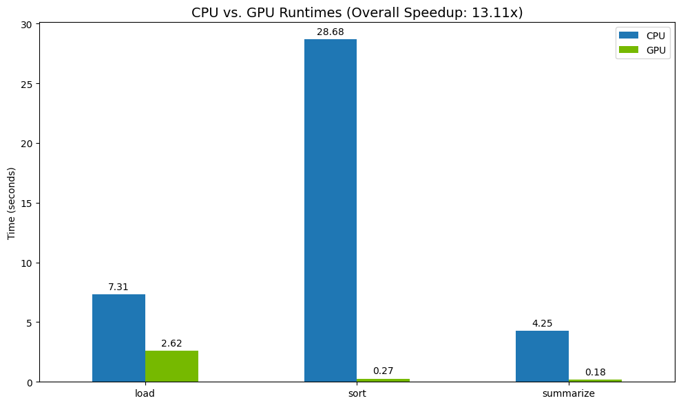
相較於 CPU，GPU 的速度明顯提升。

12. 剖析程式碼，找出瓶頸

即使使用 GPU 加速，如果 cuDF 尚未支援某些 pandas 作業，這些作業可能會回退至 CPU。這些「CPU 回退」可能會成為效能瓶頸。

為協助您找出這些區域，cudf.pandas 內建兩個剖析器。您可以使用這些工具，準確查看程式碼的哪些部分在 GPU 上執行，哪些部分則回退到 CPU。

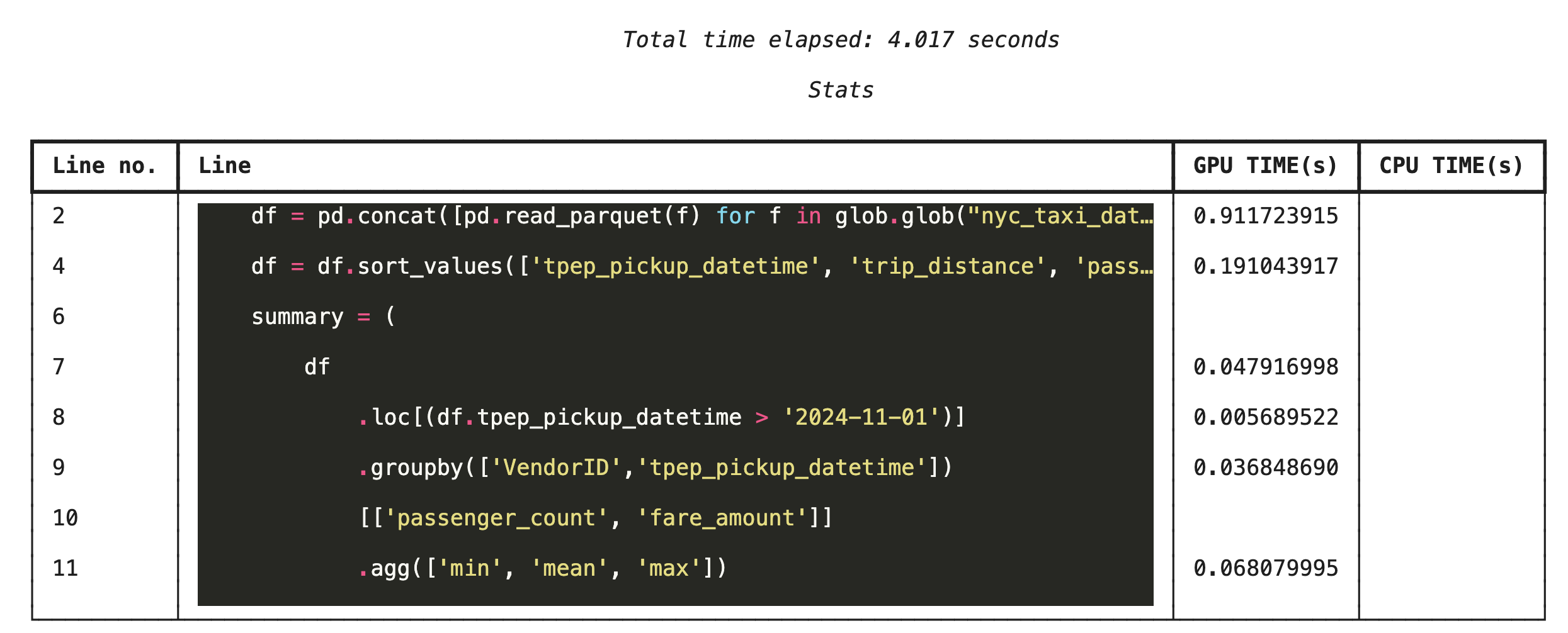
• %%cudf.pandas.profile：用於程式碼的高階摘要，以函式為單位。最適合快速瞭解哪些裝置正在執行哪些作業。
• %%cudf.pandas.line_profile：用於逐行詳細分析。這是找出程式碼中導致 CPU 回退的確切行數的最佳工具。

在筆記本儲存格頂端，使用這些剖析器做為「儲存格魔法」。

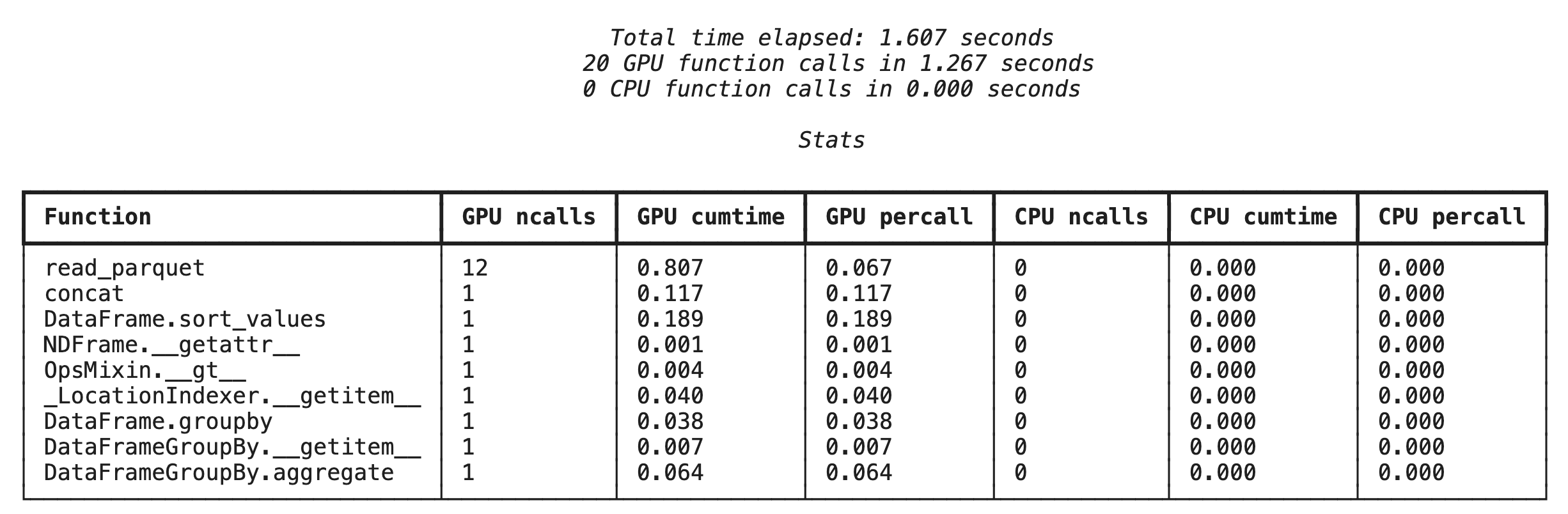
使用 %%cudf.pandas.profile 進行函式層級的剖析

首先，請在上一節的相同分析管道上執行函式層級的剖析器。輸出內容會顯示每個呼叫的函式、執行的裝置 (GPU 或 CPU)，以及呼叫次數。

%load_ext cudf.pandas
import pandas as pd
import glob

pd.DataFrame({"a": [1]})

確認 cudf.pandas 處於啟用狀態後，即可執行設定檔。

%%cudf.pandas.profile

df = pd.concat([pd.read_parquet(f) for f in glob.glob("nyc_taxi_data/*2024*.parquet")], ignore_index=True)

df = df.sort_values(['tpep_pickup_datetime', 'trip_distance', 'passenger_count'], ascending=[False, True, False])

summary = (
    df
        .loc[(df.tpep_pickup_datetime > '2024-11-01')]
        .groupby(['VendorID','tpep_pickup_datetime'])
        [['passenger_count', 'fare_amount']]
        .agg(['min', 'mean', 'max'])
)

使用 %%cudf.pandas.line_profile 逐行分析

接著，執行行層級分析器。這樣就能更精細地查看每行程式碼在 GPU 和 CPU 上執行的時間比例。這是找出特定瓶頸並加以改善最有效的方法。

%%cudf.pandas.line_profile

df = pd.concat([pd.read_parquet(f) for f in glob.glob("nyc_taxi_data/*2024*.parquet")], ignore_index=True)

df = df.sort_values(['tpep_pickup_datetime', 'trip_distance', 'passenger_count'], ascending=[False, True, False])

summary = (
    df
        .loc[(df.tpep_pickup_datetime > '2024-11-01')]
        .groupby(['VendorID','tpep_pickup_datetime'])
        [['passenger_count', 'fare_amount']]
        .agg(['min', 'mean', 'max'])
)

透過指令列進行剖析

這些剖析器也可透過指令列使用，有助於自動測試及剖析 Python 指令碼。

您可以在指令列介面中使用下列指令：

• python -m cudf.pandas --profile your_script.py
• python -m cudf.pandas --line_profile your_script.py

13. 與 Google Cloud Storage 整合

Google Cloud Storage (GCS) 是可擴充且耐用的物件儲存服務。使用 Colab Enterprise 時，GCS 是儲存資料集、模型檢查點和其他構件的絕佳位置。

Colab Enterprise 執行階段具備直接讀取及寫入 GCS bucket 資料的必要權限，且這些作業會透過 GPU 加速，發揮最大效能。

建立 GCS 值區

首先，請建立新的 GCS bucket。GCS bucket 名稱在全域範圍內不得重複，因此請在名稱後方加上 UUID。

from google.cloud import storage
import uuid

unique_suffix = uuid.uuid4().hex[:12]
bucket_name = f'nyc-taxi-codelab-{unique_suffix}'
project_id = storage.Client().project

client = storage.Client()

try:
    bucket = client.create_bucket(bucket_name)
    print(f"Successfully created bucket: gs://{bucket.name}")
except Exception as e:
    print(f"Bucket creation failed. You may already own it or the name is taken: {e}")

將資料直接寫入 GCS

現在，請直接將 DataFrame 儲存至新的 GCS bucket。如果前幾節沒有 df 變數，程式碼會先載入單一月份的資料。

%%cudf.pandas.line_profile

# Ensure the DataFrame exists before saving to GCS
if 'df' not in locals():
    print("DataFrame not found, loading a sample file...")
    df = pd.read_parquet('nyc_taxi_data/yellow_tripdata_2024-12.parquet')

print(f"Writing data to gs://{bucket_name}/nyc_taxi_data.parquet...")
df.to_parquet(f"gs://{bucket_name}/nyc_taxi_data.parquet", index=False)
print("Write operation complete.")

驗證 GCS 中的檔案

如要確認資料是否位於 GCS，請前往該 bucket。以下程式碼會建立可點選的連結。

from IPython.display import Markdown

gcs_url = f"https://console.cloud.google.com/storage/browser/{bucket_name}?project={project_id}"
Markdown(f'**[Click here to view your GCS bucket in the Google Cloud Console]({gcs_url})**')

直接從 GCS 讀取資料

最後，直接從 GCS 路徑將資料讀取至 DataFrame。這項作業也會透過 GPU 加速，讓您高速載入雲端儲存空間中的大型資料集。

%%cudf.pandas.line_profile

print(f"Reading data from gs://{bucket_name}/nyc_taxi_data.parquet...")
df_from_gcs = pd.read_parquet(f"gs://{bucket_name}/nyc_taxi_data.parquet")

df_from_gcs.head()

14. 清除

為避免 Google Cloud 帳戶產生預期外的費用，請清除您建立的資源。

刪除下載的資料：

# Permanately delete the GCS bucket
print(f"Deleting GCS bucket: gs://{bucket_name}...")
!gsutil rm -r -f gs://{bucket_name}
print("Bucket deleted.")

# Remove NYC taxi dataset on the Colab runtime
print("Deleting local 'nyc_taxi_data' directory...")
!rm -rf nyc_taxi_data
print("Local files deleted.")

關閉 Colab 執行階段

• 前往 Google Cloud 控制台的 Colab Enterprise「執行階段」頁面。
• 在「Region」(區域) 選單中，選取包含執行階段的區域。
• 選取要刪除的執行階段。
• 按一下「刪除」。
• 按一下「確認」。

刪除筆記本

• 前往 Google Cloud 控制台的 Colab Enterprise「我的筆記本」頁面。
• 在「Region」(區域) 選單中，選取包含筆記本的區域。
• 選取要刪除的記事本。
• 按一下「刪除」。
• 按一下「確認」。

15. 恭喜

恭喜！您已在 Colab Enterprise 中使用 NVIDIA cuDF，成功加速 pandas 分析工作流程。您已學會如何設定啟用 GPU 的執行階段、啟用 cudf.pandas 以加速執行作業 (無需變更程式碼)、剖析程式碼找出瓶頸，以及與 Google Cloud Storage 整合。

參考文件

• Colab Enterprise 說明文件
• NVIDIA cuDF 說明文件