Accelerated Machine Learning with Google Cloud and NVIDIA

1. Introduction

In this codelab, you will learn how to accelerate your data science and machine learning workflows on large datasets using NVIDIA GPUs and open-source libraries on Google Cloud. You will start by setting up your infrastructure, then explore how to apply GPU acceleration.

You will focus on the data science lifecycle, from data preparation with pandas to model training with scikit-learn and XGBoost. You will learn how to accelerate these tasks using NVIDIA's cuDF and cuML libraries. The best part is you can get this GPU acceleration without changing your existing pandas or scikit-learn code.

What you'll learn

• Understand Colab Enterprise on Google Cloud.
• Customize a Colab runtime environment with specific GPU and memory configurations.
• Apply GPU acceleration to predict tip amounts using millions of records from a NYC Taxi dataset.
• Accelerate pandas with zero code changes using NVIDIA's cuDF library.
• Accelerate scikit-learn with zero code changes using NVIDIA's cuML library and GPUs.
• Profile your code to identify and optimize performance constraints.

Note: This codelab is designed for practitioners who already understand standard machine learning steps and want to learn how to accelerate them. It focuses on the application of GPU acceleration to a realistic, end-to-end workflow rather than teaching the underlying machine learning theory.

If you are looking for a more basic introduction focused on data analytics rather than machine learning, check out the Accelerated Data Analytics with GPUs codelab.

2. Why accelerate machine learning?

The need for faster iteration in ML

Data preparation is time-consuming, and model training or evaluation can take even longer as datasets grow. Training models like random forests or XGBoost on millions of rows with a CPU can take hours or days.

Using GPUs accelerates these training runs with libraries like cuML and GPU-accelerated XGBoost. This acceleration lets you:

• Iterate faster: Test new features and hyperparameters quickly.
• Train on full datasets: Use your complete data instead of downsampling for better accuracy.
• Reduce costs: Complete heavy workloads in less time to lower compute costs.

3. Setup and requirements

Potential costs

This codelab uses Google Cloud resources, including Colab Enterprise runtimes with NVIDIA L4 GPUs. Please be aware of potential charges and follow the Clean Up section at the end of the codelab to shut down resources and avoid ongoing billing. For detailed pricing information, refer to Colab Enterprise pricing and GPU pricing.

Before you begin

Intermediate familiarity with Python, pandas, scikit-learn, and standard machine learning practices (like cross-validation/ensembling) is assumed.

1. In the Google Cloud Console, on the project selector page, select or create a Google Cloud project.
2. Make sure that billing is enabled for your Google Cloud project.

Enable the APIs

To use Colab Enterprise, you must first enable the necessary APIs.

1. Open Google Cloud Shell by clicking the Cloud Shell icon in the top right of the Google Cloud Console.

2. In Cloud Shell, set your project ID by replacing PROJECT_ID with your project ID:

gcloud config set project <PROJECT_ID>

3. Run the following command to enable the necessary APIs:

gcloud services enable \
    compute.googleapis.com \
    dataform.googleapis.com \
    notebooks.googleapis.com \
    aiplatform.googleapis.com

On successful execution, you should see a message similar to the one shown below:

Operation "operations/..." finished successfully.

4. Choosing a notebook environment

While many data scientists are familiar with Colab for personal projects, Colab Enterprise provides a secure, collaborative, and integrated notebook experience designed for businesses.

On Google Cloud, you have two primary choices for managed notebook environments: Colab Enterprise and Vertex AI Workbench. The right choice depends on your project's priorities.

When to use Vertex AI Workbench

Choose Vertex AI Workbench when your priority is control and deep customization. It's the ideal choice if you need to:

• Manage the underlying infrastructure and machine lifecycle.
• Use custom containers and network configurations.
• Integrate with MLOps pipelines and custom lifecycle tooling.

When to use Colab Enterprise

Choose Colab Enterprise when your priority is fast setup, ease of use, and secure collaboration. It is a fully managed solution that allows your team to focus on analysis instead of infrastructure.

Colab Enterprise helps you:

• Develop data science workflows that are closely tied to your data warehouse. You can open and manage your notebooks directly in BigQuery Studio.
• Train machine learning models and integrate with MLOps tools in Vertex AI.
• Enjoy a flexible and unified experience. A Colab Enterprise notebook created in BigQuery can be opened and run in Vertex AI, and vice versa.

Today's lab

This Codelab uses Colab Enterprise for accelerated machine learning.

To learn more about the differences, see the official documentation on choosing the right notebook solution.

5. Configure a runtime template

In Colab Enterprise, connect to a runtime based on a pre-configured runtime template.

A runtime template is a reusable configuration that specifies the environment for your notebook, including:

• Machine type (CPU, memory)
• Accelerator (GPU type and count)
• Disk size and type
• Network settings and security policies
• Automatic idle shutdown rules

Why runtime templates are useful

• Consistency: You and your team get the same environment to ensure work is repeatable.
• Security: Templates enforce organization security policies.
• Cost management: Resources are pre-sized in the template to help prevent accidental costs.

Create a runtime template

Set up a reusable runtime template for the lab.

1. In the Google Cloud Console, go to the Navigation Menu > Vertex AI > Colab Enterprise.

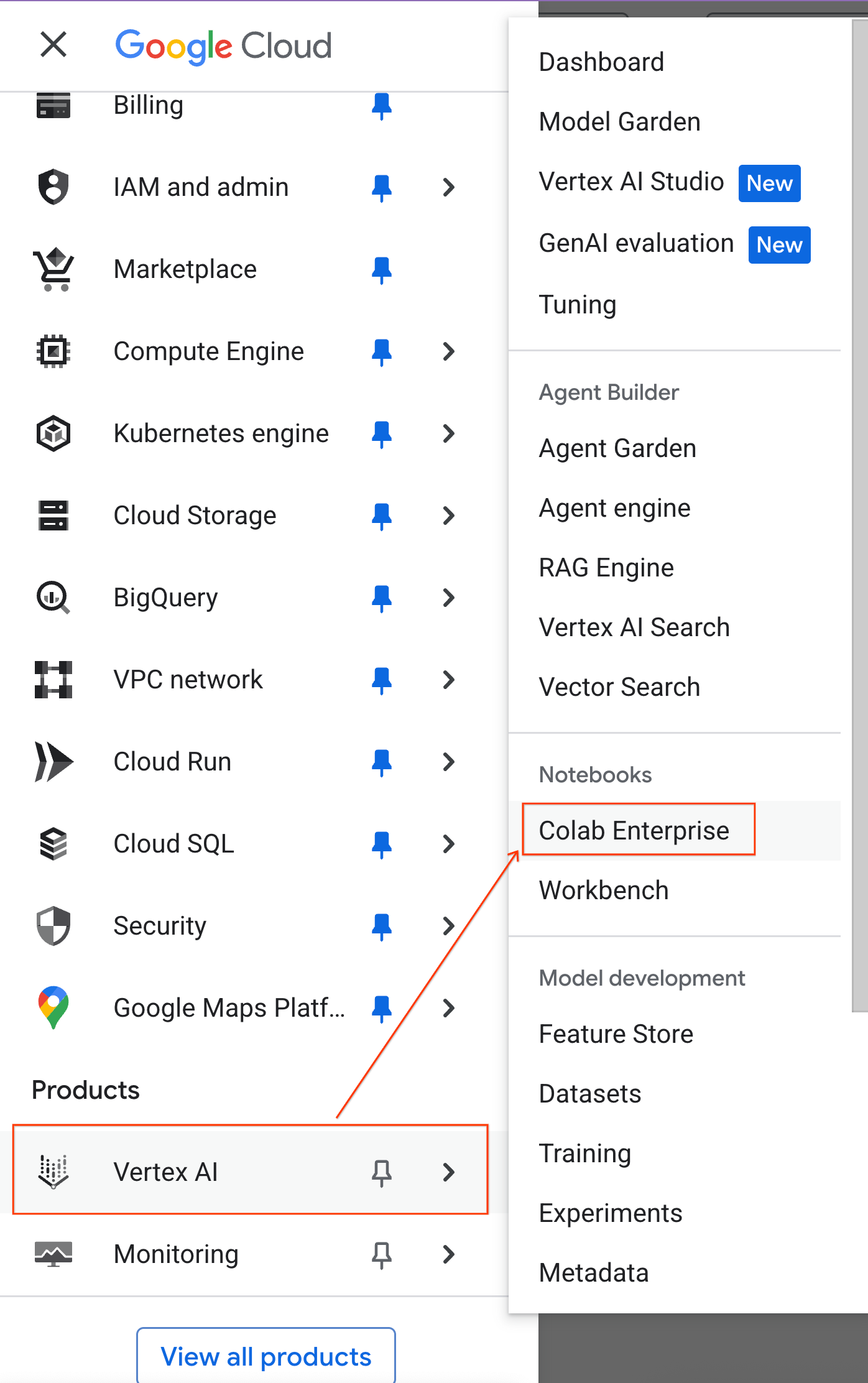
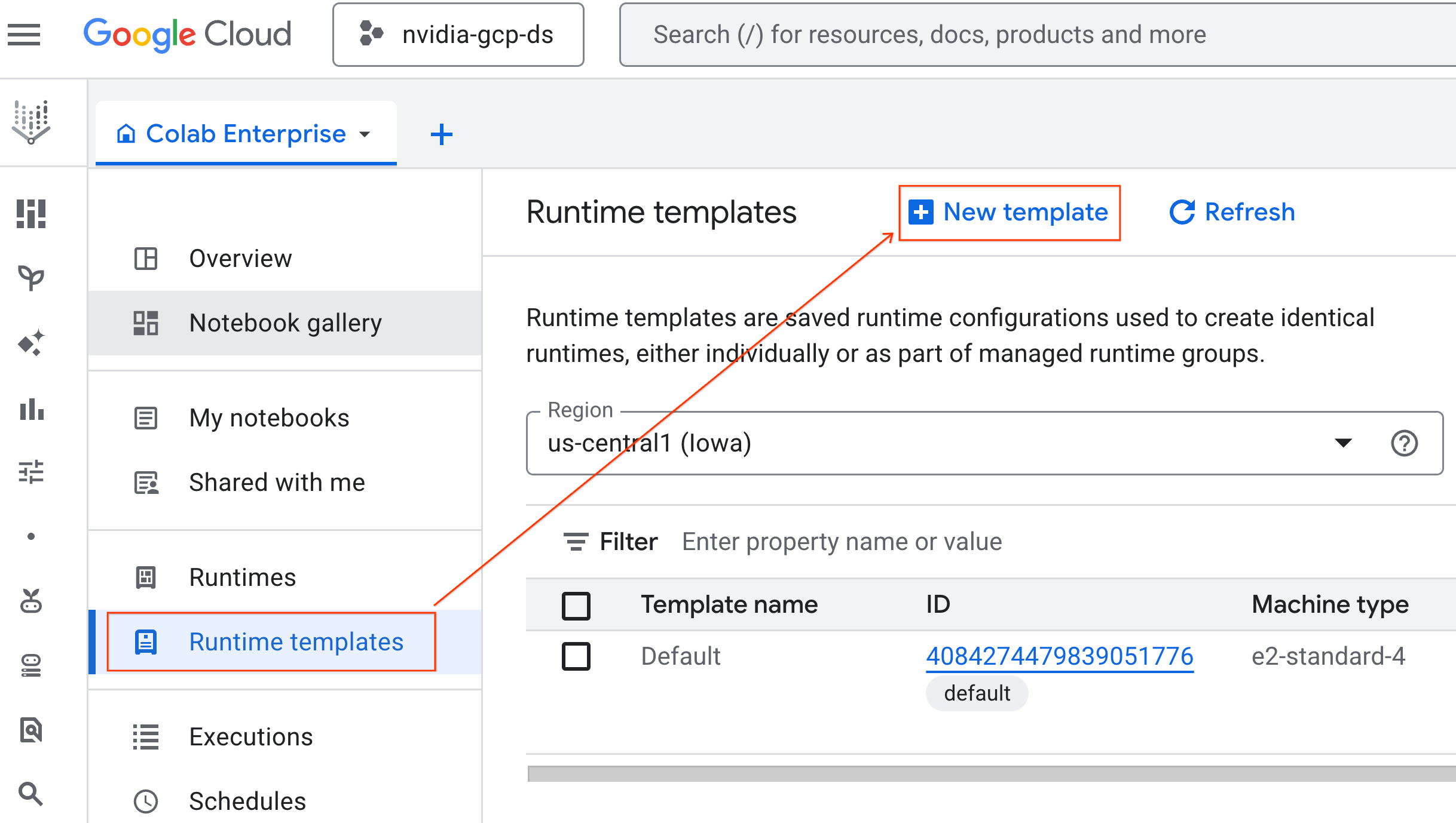
2. From Colab Enterprise, click Runtime templates and then select New Template.

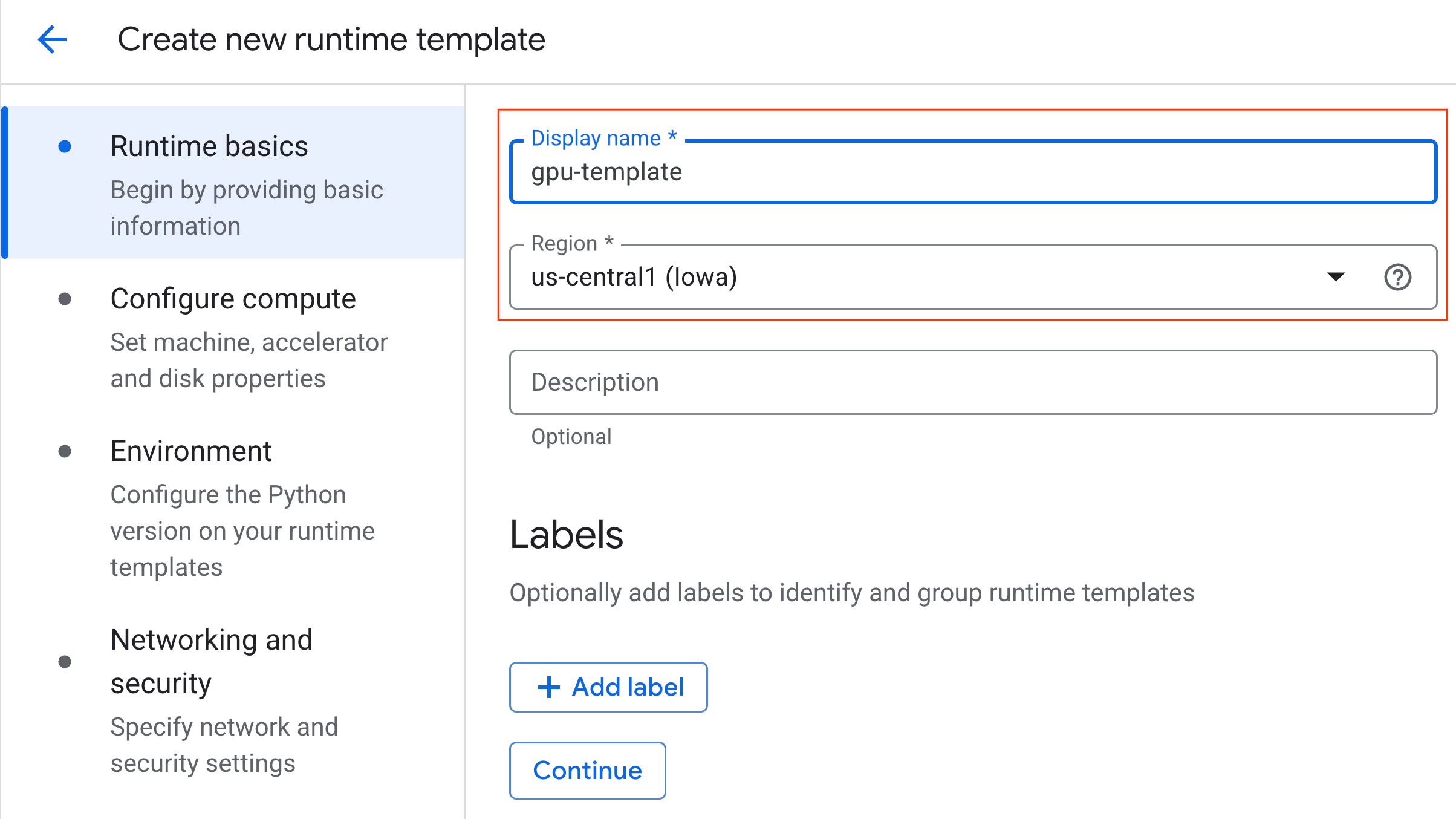
3. Under Runtime basics:
   • Set the Display name as gpu-template.
   • Set your preferred Region.

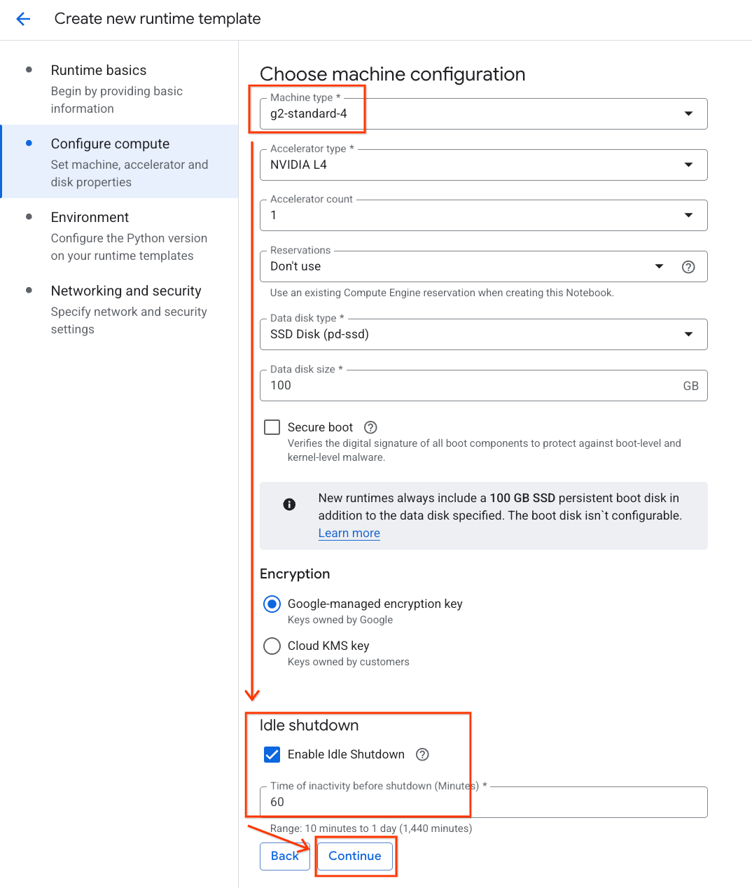
4. Under Configure compute:
   • Set the Machine type to g2-standard-4.
   • Keep the default Accelerator Type as NVIDIA L4 with an Accelerator count of 1.
   • Change the Idle shutdown to 60 minutes.
   • Click Continue.

5. Under Environment:
   • Set the Environment to Python 3.11

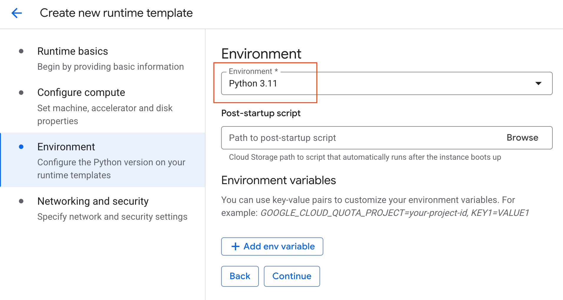
6. Click Create to save the runtime template. Your Runtime templates page should now display the new template.

6. Start a runtime

With your template ready, you can create a new runtime.

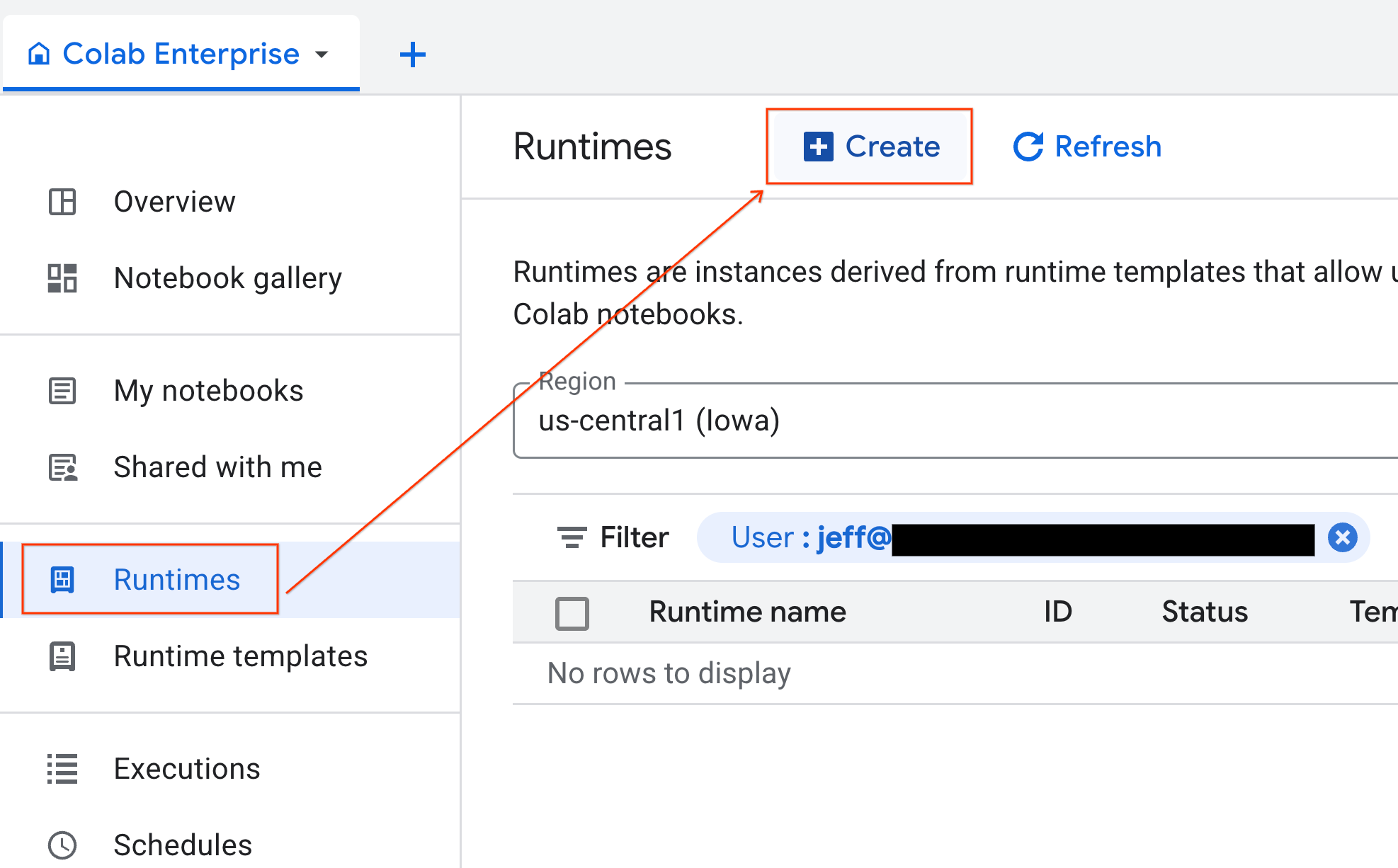
1. From Colab Enterprise, click Runtimes and then select Create.

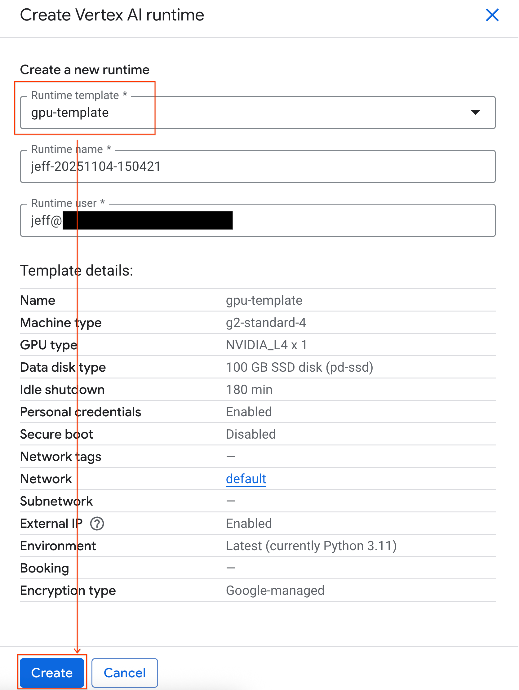
2. Under Runtime template, select the gpu-template option. Click Create and wait for the runtime to boot up.

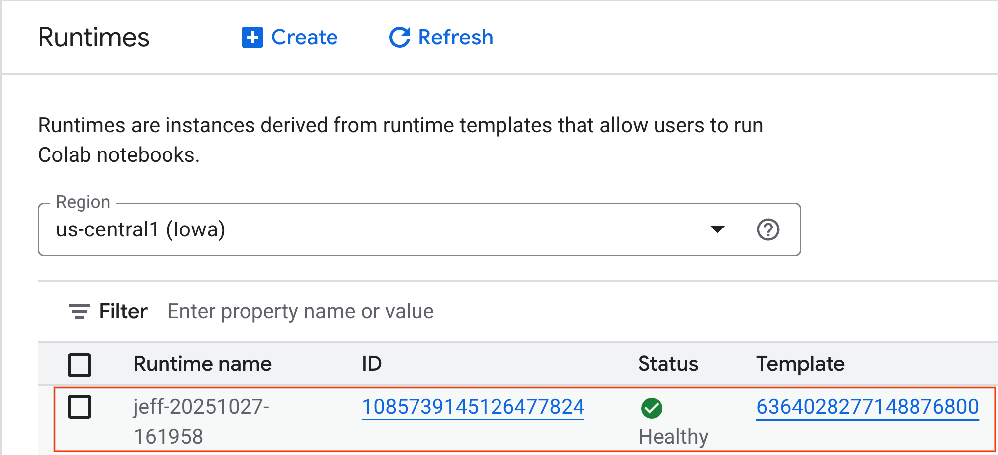
3. After a few minutes, you will see the runtime available.

Note: If you receive a failure notification, try again in a few minutes or in a different region. The failure is likely due to high GPU demand.

7. Set up the notebook

Now that your infrastructure is running, you need to import the lab notebook and connect it to your runtime.

Import the notebook

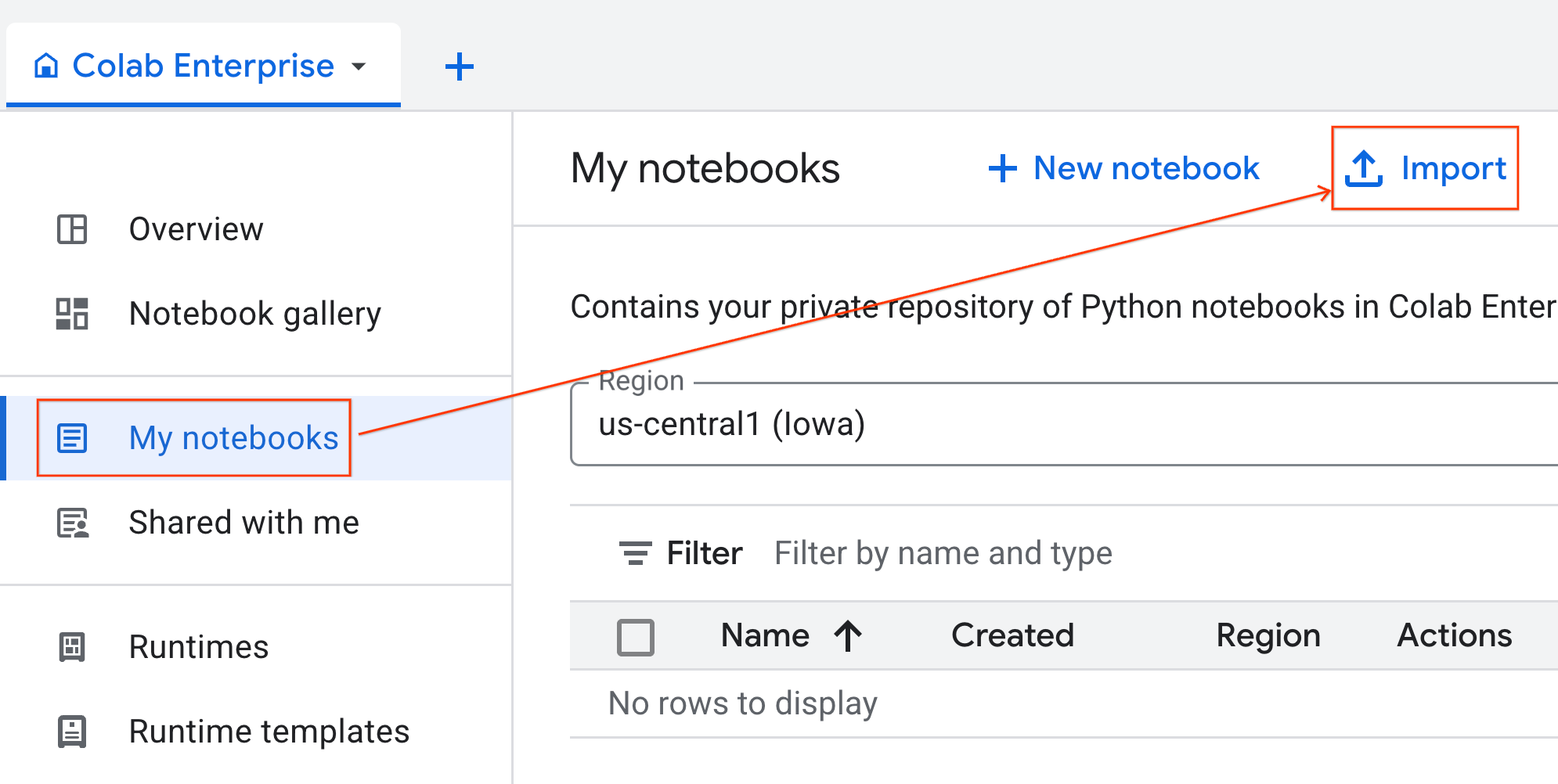
1. From Colab Enterprise, click My notebooks and then click Import.

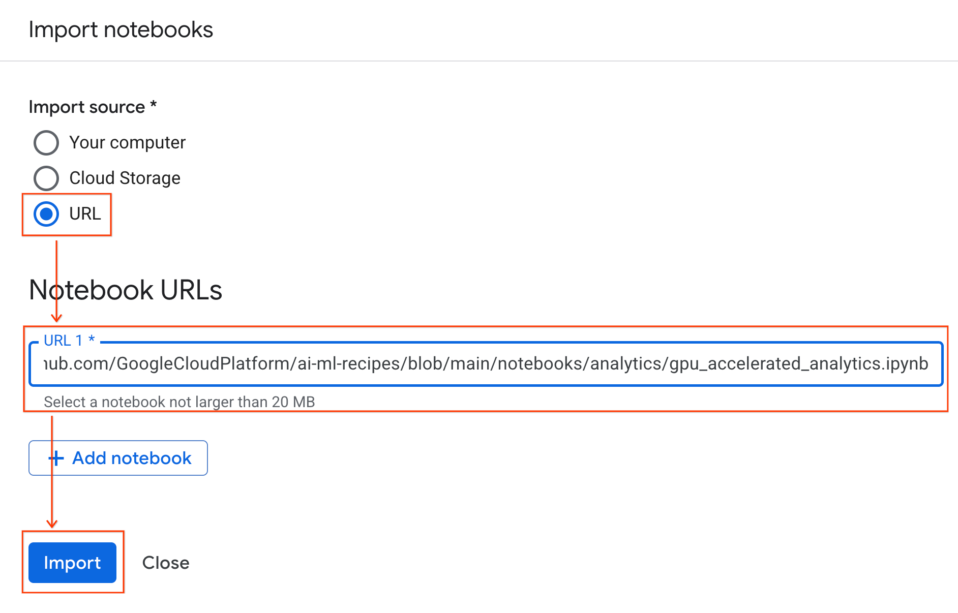
2. Select the URL radio button and input the following URL:

https://github.com/GoogleCloudPlatform/ai-ml-recipes/blob/main/notebooks/regression/gpu_accelerated_regression/gpu_accelerated_regression.ipynb

3. Click Import. Colab Enterprise will copy the notebook from GitHub into your environment.

Connect to the runtime

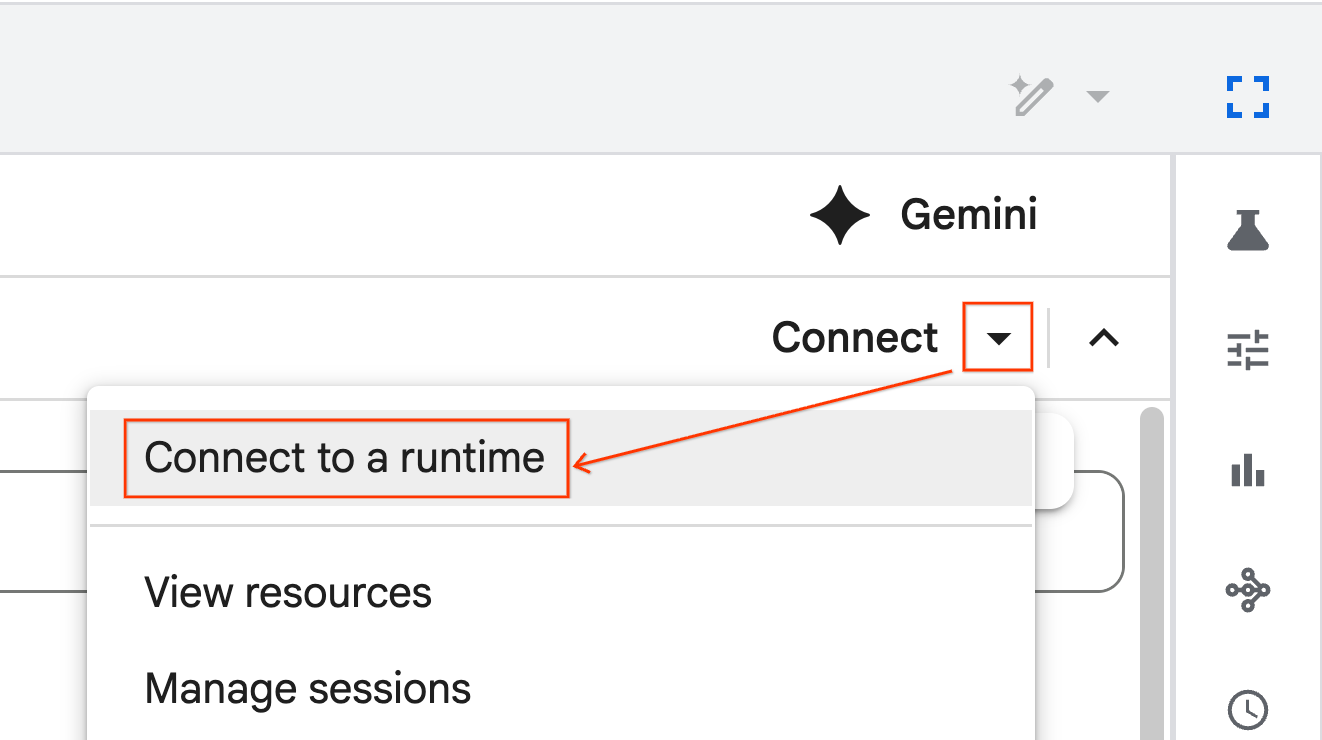
1. Open the newly imported notebook.
2. Click the down arrow next to Connect.
3. Select Connect to a runtime.

4. Use the dropdown and select the runtime you previously created.
5. Click Connect.

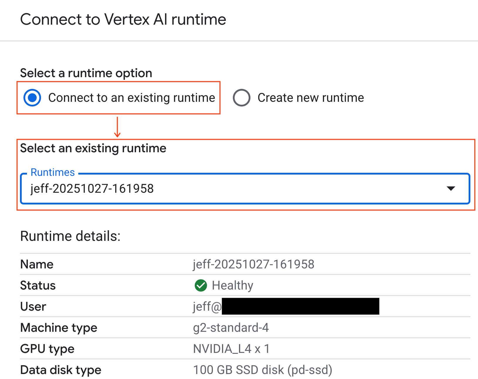
Your notebook is now connected to a GPU-enabled runtime.

Built-in dependencies

One benefit of using Colab Enterprise is that it comes pre-installed with the libraries you need. You don't need to manually install or manage dependencies like cuDF, cuML, or XGBoost for this lab.

Note: Code snippets in future sections are for explanations only. Your notebook contains all necessary code and you do not need to copy and paste from the Codelab.

8. Prepare the NYC taxi dataset

This codelab uses NYC Taxi & Limousine Commission (TLC) Trip Record Data. The dataset contains trip records from yellow taxis in New York City, including:

• Pick-up and drop-off dates, times, and locations
• Trip distances
• Itemized fare amounts
• Passenger counts
• Tip amounts (this is what we'll predict!)

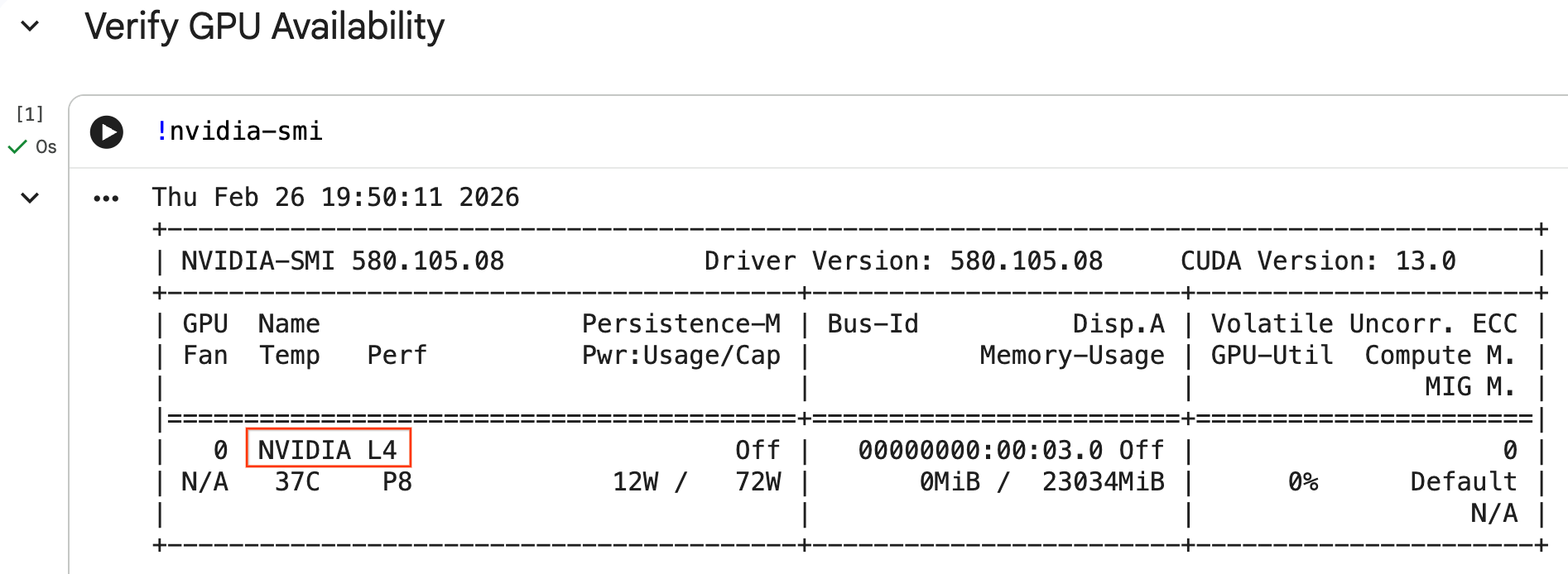
Configure GPU and confirm availability

You can confirm the GPU is recognized by running the nvidia-smi command. It displays the driver version and GPU details (such as the NVIDIA L4).

nvidia-smi

The cell should return the GPU attached to your runtime, similar to the following:

Download the data

Download the trip data for 2024.

Note: We download the entire year, but the notebook only loads the first month's data to keep execution times fast. Feel free to experiment with the larger dataset later.

from tqdm import tqdm
import requests
import time
import os

YEAR = 2024
DATA_DIR = "nyc_taxi_data"

os.makedirs(DATA_DIR, exist_ok=True)
print(f"Checking/Downloading files for {YEAR}...")

for month in tqdm(range(1, 13), unit="file"):
    file_name = f"yellow_tripdata_{YEAR}-{month:02d}.parquet"
    local_path = os.path.join(DATA_DIR, file_name)
    url = f"https://d37ci6vzurychx.cloudfront.net/trip-data/{file_name}"

    if not os.path.exists(local_path):
        try:
            with requests.get(url, stream=True) as response:
                response.raise_for_status()
                with open(local_path, 'wb') as f:
                    for chunk in response.iter_content(chunk_size=8192):
                        f.write(chunk)
            time.sleep(1)
        except requests.exceptions.HTTPError as e:
            print(f"\nSkipping {file_name}: {e}")
            if os.path.exists(local_path):
                os.remove(local_path)

print("\nDownload complete.")

Accelerate pandas with NVIDIA cuDF

The pandas library runs on the CPU and can be slow with large datasets. The NVIDIA %load_ext cudf.pandas magic command dynamically patches pandas to use GPU acceleration, falling back to the CPU if needed.

We use this magic command instead of a standard import because it provides ‘zero code change' acceleration. You don't have to rewrite any of your existing code. A similar command, %load_ext cuml.accel, does the exact same thing for scikit-learn models! This works in any Jupyter environment with a compatible NVIDIA GPU, not just Colab Enterprise.

%load_ext cudf.pandas

To verify it is active, import pandas and check its type:

import pandas as pd

pd

The output will confirm you are now using the cudf.pandas module.

Load and clean data

With cudf.pandas active, load the Parquet files and execute data cleaning. This process automatically runs on the GPU.

import glob

# Load data into memory
df = pd.concat(
    [pd.read_parquet(f) for f in glob.glob("nyc_taxi_data/*-01.parquet")],
    ignore_index=True
)

# Filter for valid trips. We filter for payment_type=1 (credit card)
# because tip amounts are only reliably recorded for credit card transactions.
df = df[
    (df['fare_amount'] > 0) & (df['fare_amount'] < 500) &
    (df['trip_distance'] > 0) & (df['trip_distance'] < 100) &
    (df['tip_amount'] >= 0) & (df['tip_amount'] < 100) &
    (df['payment_type'] == 1)
].copy()

# Downcast numeric columns to save memory
float_cols = df.select_dtypes(include=['float64']).columns
df[float_cols] = df[float_cols].astype('float32')

int_cols = df.select_dtypes(include=['int64']).columns
df[int_cols] = df[int_cols].astype('int32')

Feature Engineering

Create derived features from the pickup datetime. The notebook contains other features used in later steps.

import numpy as np

# Time Features
df['hour'] = df['tpep_pickup_datetime'].dt.hour
df['dow'] = df['tpep_pickup_datetime'].dt.dayofweek
df['is_weekend'] = (df['dow'] >= 5).astype(int)
df['is_rush_hour'] = (
    ((df['hour'] >= 7) & (df['hour'] <= 9)) |
    ((df['hour'] >= 17) & (df['hour'] <= 19))
).astype(int)

...
# Other features
...

9. Train Individual Models with Cross-Validation

To show how the GPU can accelerate machine learning, you will train three different types of regression models to predict the tip_amount of a taxi trip.

Accelerate scikit-learn with NVIDIA cuML

Run scikit-learn algorithms on the GPU using NVIDIA cuML without changing API calls. First, load the cuml.accel extension.

%load_ext cuml.accel

Setup features and targets

Identify the features you want the model to learn from and split out the target column (tip_amount).

feature_cols = [
    'trip_distance', 'fare_amount', 'passenger_count',
    'hour', 'dow', 'is_weekend', 'is_rush_hour',
    'fare_log', 'fare_decimal', 'is_round_fare',
    'route_frequency', 'pu_tip_mean', 'pu_tip_std',
    'PULocationID', 'DOLocationID'
]

X = df[feature_cols].fillna(df[feature_cols].median())
y = df['tip_amount'].copy()

Set up cross-validation splits to robustly evaluate model performance.

Note: Cross-validation requires training a model multiple times across different data splits. Because this process is inherently computationally expensive, it represents an ideal scenario for GPU acceleration.

from sklearn.model_selection import KFold
import numpy as np
import time
from sklearn.metrics import mean_squared_error
from tqdm.notebook import tqdm

n_splits = 3
kf = KFold(n_splits=n_splits, shuffle=True, random_state=42)

1. XGBoost

XGBoost is natively GPU-accelerated. Pass tree_method='hist' and device='cuda' to use the GPU during training.

import xgboost as xgb

start_time = time.perf_counter()

def train_xgb_cv(X, y):
    rmses = []
    preds_all = np.zeros(len(y))
    for train_idx, val_idx in tqdm(kf.split(X), total=n_splits):
        X_train, X_val = X.iloc[train_idx], X.iloc[val_idx]
        y_train, y_val = y.iloc[train_idx], y.iloc[val_idx]
        
        # XGBoost handles GPU natively when tree_method='hist' and device='cuda'
        model = xgb.XGBRegressor(
            objective='reg:squarederror',
            max_depth=5,
            learning_rate=0.1,
            n_estimators=100,
            tree_method='hist',
            device='cuda',
            random_state=42
        )
        model.fit(X_train, y_train)
        
        preds = model.predict(X_val)
        preds_all[val_idx] = preds
        rmses.append(np.sqrt(mean_squared_error(y_val, preds)))
        
    return np.mean(rmses), preds_all

xgb_rmse, xgb_preds = train_xgb_cv(X, y)
print(f"\n{'XGBoost RMSE:':<20} ${xgb_rmse:.4f}")
print(f"{'Time:':<20} {time.perf_counter() - start_time:.2f} seconds")

Note: If you do not specify tree_method='hist' along with device='cuda', XGBoost might default to an exact tree method, which can be slower or exhaust memory limits on larger datasets.

2. Linear Regression

Train a linear regression model. With %load_ext cuml.accel active, LinearRegression maps to its GPU equivalent automatically.

from sklearn.linear_model import LinearRegression
from sklearn.preprocessing import StandardScaler

start_time = time.perf_counter()

def train_linreg_cv(X, y):
    rmses = []
    preds_all = np.zeros(len(y))
    for train_idx, val_idx in tqdm(kf.split(X), total=n_splits):
        X_train, X_val = X.iloc[train_idx], X.iloc[val_idx]
        y_train, y_val = y.iloc[train_idx], y.iloc[val_idx]

        # Scale features
        scaler = StandardScaler()
        X_train_scaled = scaler.fit_transform(X_train)
        X_val_scaled = scaler.transform(X_val)

        # Automatically accelerated by cuML
        model = LinearRegression()
        model.fit(X_train_scaled, y_train)

        preds = model.predict(X_val_scaled)
        preds_all[val_idx] = preds
        rmses.append(np.sqrt(mean_squared_error(y_val, preds)))

    return np.mean(rmses), preds_all

linreg_rmse, linreg_preds = train_linreg_cv(X, y)
print(f"\n{'Linear Reg RMSE:':<20} ${linreg_rmse:.4f}")
print(f"{'Time:':<20} {time.perf_counter() - start_time:.2f} seconds")

3. Random Forest

Train an ensemble model using RandomForestRegressor. Tree-based models are often slow to train on the CPU, but GPU acceleration processes millions of rows faster.

from sklearn.ensemble import RandomForestRegressor

start_time = time.perf_counter()

def train_rf_cv(X, y):
    rmses = []
    preds_all = np.zeros(len(y))
    for train_idx, val_idx in tqdm(kf.split(X), total=n_splits):
        X_train, X_val = X.iloc[train_idx], X.iloc[val_idx]
        y_train, y_val = y.iloc[train_idx], y.iloc[val_idx]

        # Automatically accelerated by cuML
        model = RandomForestRegressor(
            n_estimators=100,
            max_depth=10,
            n_jobs=-1,
            max_features='sqrt',
            random_state=42
        )
        model.fit(X_train, y_train)

        preds = model.predict(X_val)
        preds_all[val_idx] = preds
        rmses.append(np.sqrt(mean_squared_error(y_val, preds)))

    return np.mean(rmses), preds_all

rf_rmse, rf_preds = train_rf_cv(X, y)
print(f"\n{'Random Forest RMSE:':<20} ${rf_rmse:.4f}")
print(f"{'Time:':<20} {time.perf_counter() - start_time:.2f} seconds")

10. Evaluate the End-to-End Pipeline

Combine the predictions from the three models using a simple linear ensemble. This typically provides a slight accuracy lift over individual models.

Note: We've included standard data preparation and ensembling steps to provide a realistic, end-to-end ML pipeline. You will see how cudf.pandas and cuml.accel handle these standard practices without rewriting your code.

Fit a linear regression on the predictions to find the optimal weights:

ensemble_weights = LinearRegression(positive=True, fit_intercept=False).fit(
    np.c_[xgb_preds, rf_preds, linreg_preds], y
).coef_

# Normalize weights
ensemble_weights = ensemble_weights / ensemble_weights.sum()

ensemble_preds = np.c_[xgb_preds, rf_preds, linreg_preds] @ ensemble_weights
ensemble_rmse = np.sqrt(mean_squared_error(y, ensemble_preds))

Compare the results to see the ensemble lift:

print(f"\n{'Model':<20} {'RMSE':>10}")
print("-" * 32)
print(f"{'Linear Regression':<20} ${linreg_rmse:>9.4f}")
print(f"{'Random Forest':<20} ${rf_rmse:>9.4f}")
print(f"{'XGBoost':<20} ${xgb_rmse:>9.4f}")
print("-" * 32)
print(f"{'Ensemble':<20} ${ensemble_rmse:>9.4f}")
print(f"\nEnsemble lift: ${xgb_rmse - ensemble_rmse:.4f}")

11. Compare CPU vs. GPU performance

To benchmark the performance difference properly, you will restart the kernel to ensure a clean execution state, run the entire data science pipeline on the CPU, and then run it again on the GPU.

Restart the kernel

Run the IPython.Application.instance().kernel.do_shutdown(True) command to restart the kernel and release memory.

import IPython
IPython.Application.instance().kernel.do_shutdown(True)

Define the data science pipeline

Wrap the core workflow (loading data, cleaning, feature engineering, and model training) into a single function. This function accepts a pandas module pd_module and an use_gpu argument to switch between environments.

Note: For a clear CPU vs. GPU comparison, this function uses fewer features and skips cross-validation to focus on core pipeline steps.

def run_ml_pipeline(pd_module, use_gpu=False):
    import time
    import glob
    import numpy as np
    from sklearn.ensemble import RandomForestRegressor
    import xgboost as xgb

    timings = {}

    # 1. Load Data
    t0 = time.perf_counter()
    df = pd_module.concat(
        [pd_module.read_parquet(f) for f in glob.glob("nyc_taxi_data/*-01.parquet")],
        ignore_index=True
    )
    timings['Load Data'] = time.perf_counter() - t0

    # 2. Clean Data
    t0 = time.perf_counter()
    # Filter for payment_type=1 (credit card) because tip amounts
    # are only reliably recorded for credit card transactions.
    df = df[
        (df['fare_amount'] > 0) & (df['fare_amount'] < 500) &
        (df['trip_distance'] > 0) & (df['trip_distance'] < 100) &
        (df['tip_amount'] >= 0) & (df['tip_amount'] < 100) &
        (df['payment_type'] == 1)
    ].copy()

    # Downcast numeric columns to save memory
    float_cols = df.select_dtypes(include=['float64']).columns
    df[float_cols] = df[float_cols].astype('float32')
    int_cols = df.select_dtypes(include=['int64']).columns
    df[int_cols] = df[int_cols].astype('int32')
    timings['Clean Data'] = time.perf_counter() - t0

    # 3. Feature Engineering
    t0 = time.perf_counter()
    df['hour'] = df['tpep_pickup_datetime'].dt.hour
    df['dow'] = df['tpep_pickup_datetime'].dt.dayofweek
    df['is_weekend'] = (df['dow'] >= 5).astype(int)
    df['fare_log'] = np.log1p(df['fare_amount'])
    timings['Feature Engineering'] = time.perf_counter() - t0

    # 4. Modeling Prep
    feature_cols = ['trip_distance', 'fare_amount', 'passenger_count', 'hour', 'dow', 'is_weekend', 'fare_log']
    X = df[feature_cols].fillna(df[feature_cols].median())
    y = df['tip_amount'].copy()

    # Free memory
    del df
    import gc
    gc.collect()

    # 5. Train Random Forest
    t0 = time.perf_counter()
    rf_model = RandomForestRegressor(
        n_estimators=100,
        max_depth=10,
        n_jobs=-1,
        max_features='sqrt',
        random_state=42
    ).fit(X, y)
    timings['Train Random Forest'] = time.perf_counter() - t0

    # 6. Train XGBoost
    t0 = time.perf_counter()
    params = {
        'objective': 'reg:squarederror', 
        'max_depth': 5,
        'n_estimators': 100,
        'random_state': 42
    }
    if use_gpu:
        params['device'] = 'cuda'
        params['tree_method'] = 'hist'
    xgb_model = xgb.XGBRegressor(**params).fit(X, y)
    timings['Train XGBoost'] = time.perf_counter() - t0

    del X
    del y
    gc.collect()

    return timings

Run on your CPU

Call the pipeline using standard CPU pandas.

import pandas as pd

print("Running pipeline on CPU...")
cpu_times = run_ml_pipeline(pd, use_gpu=False)
print("CPU Execution Finished.")

Run on your GPU

Load the NVIDIA library extensions, pass the accelerated cudf.pandas module to the pipeline, and set your XGBoost device to cuda internally.

import IPython.core.magic
if not hasattr(IPython.core.magic, 'output_can_be_silenced'):
    IPython.core.magic.output_can_be_silenced = lambda x: x

%load_ext cudf.pandas
%load_ext cuml.accel
import pandas as pd

print("Running pipeline on GPU...")
gpu_times = run_ml_pipeline(pd, use_gpu=True)
print("GPU Execution Finished.")

Visualize the performance speedup

Visualize the timings using matplotlib. The results show time saved during data processing and model training when using GPUs.

import matplotlib.pyplot as plt
import numpy as np

labels = list(cpu_times.keys())
cpu_values = list(cpu_times.values())
gpu_values = list(gpu_times.values())

x = np.arange(len(labels))
width = 0.35

fig, ax = plt.subplots(figsize=(10, 6))
rects1 = ax.bar(x - width/2, cpu_values, width, label='CPU', color='#4285F4')
rects2 = ax.bar(x + width/2, gpu_values, width, label='GPU', color='#76B900')

ax.set_ylabel('Execution Time (seconds)')
ax.set_title('NYC Taxi ML Pipeline: CPU vs. GPU Performance')
ax.set_xticks(x)
ax.set_xticklabels(labels, rotation=45, ha="right")
ax.legend()

# Add data labels
def autolabel(rects):
    for rect in rects:
        height = rect.get_height()
        ax.annotate(f'{height:.2f}s',
                    xy=(rect.get_x() + rect.get_width() / 2, height),
                    xytext=(0, 3),  # 3 points vertical offset
                    textcoords="offset points",
                    ha='center', va='bottom', fontsize=9)
autolabel(rects1)
autolabel(rects2)

plt.tight_layout()
plt.show()

# Calculate overall speedup
total_cpu_time = sum(cpu_values)
total_gpu_time = sum(gpu_values)
overall_speedup = total_cpu_time / total_gpu_time
print(f"\nOverall Pipeline Speedup: {overall_speedup:.2f}x faster on GPU!")

You should see something like:

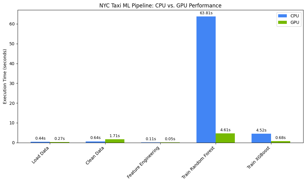
This chart illustrates the significant performance advantage of the GPU across the entire data science workflow. You should expect to see the most dramatic time savings unlocked during the computationally intensive model training phases for algorithms like Random Forest and XGBoost.

12. Profile your code to find performance constraints

When using cudf.pandas, most functions run on the GPU. If a specific operation is not yet supported by cuDF, execution temporarily falls back to the CPU. NVIDIA provides two built-in Jupyter magic commands to identify these fallbacks.

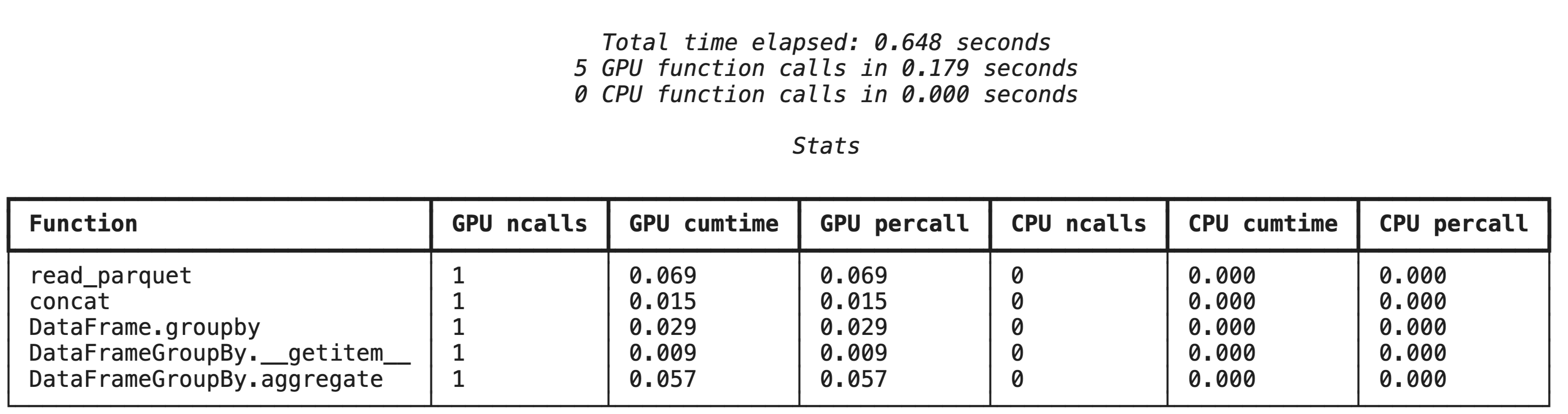
High-level profiling with %%cudf.pandas.profile

The %%cudf.pandas.profile magic command provides a summary of which functions ran on the GPU or CPU.

%%cudf.pandas.profile

import glob
import pandas as pd

df = pd.concat([pd.read_parquet(f) for f in glob.glob("nyc_taxi_data/*-01.parquet")], ignore_index=True)

summary = (
    df
      .groupby(['PULocationID', 'payment_type'])
      [['passenger_count', 'fare_amount', 'tip_amount']]
      .agg(['min', 'mean', 'max'])
)

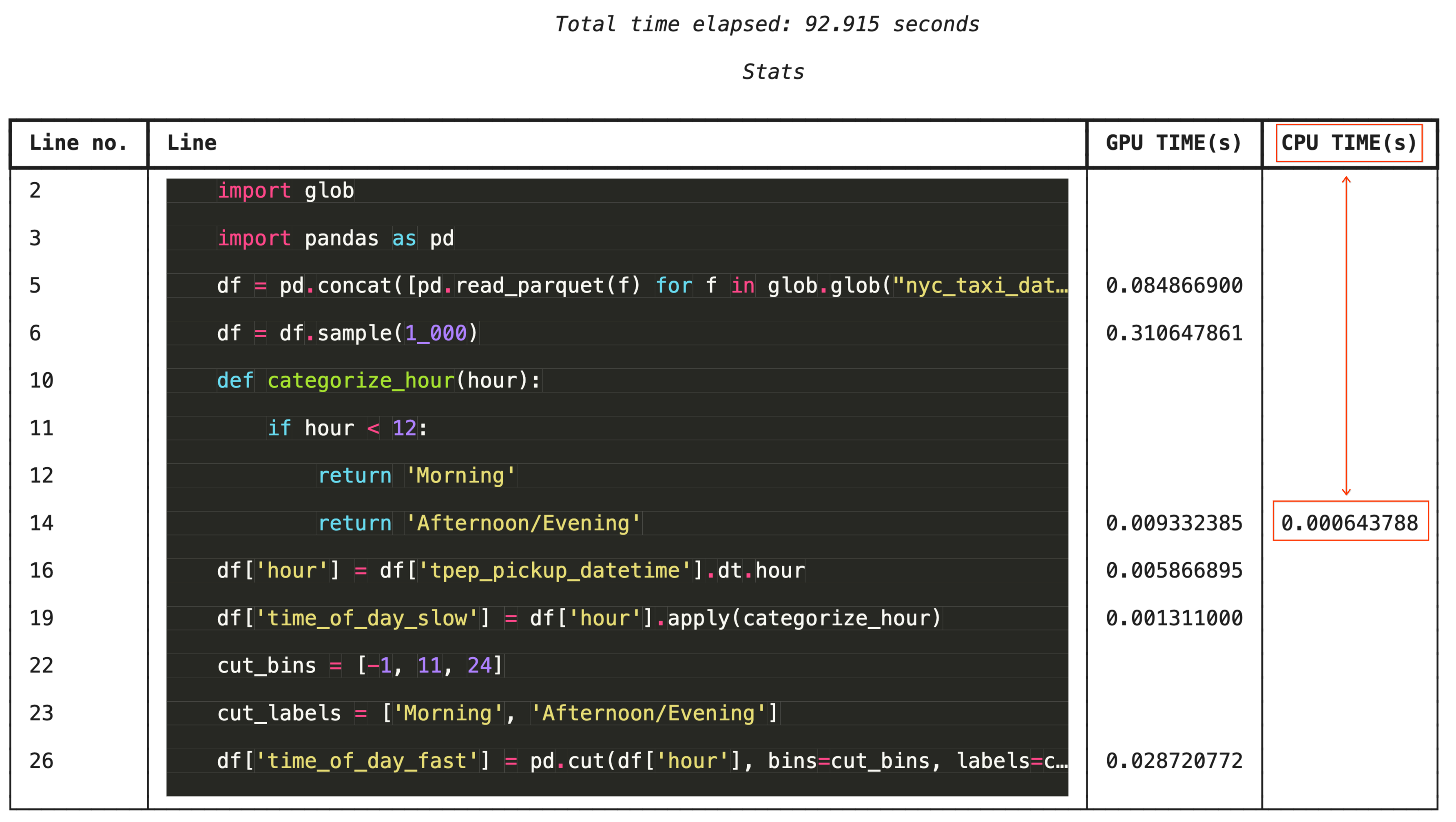
Line-by-line profiling with %%cudf.pandas.line_profile

For granular troubleshooting, %%cudf.pandas.line_profile annotates each line of code with the number of times it executed on the GPU versus the CPU.

%%cudf.pandas.line_profile

import glob
import pandas as pd

df = pd.concat([pd.read_parquet(f) for f in glob.glob("nyc_taxi_data/*-01.parquet")], ignore_index=True)
df = df.sample(1_000)

# Iterating row-by-row or using custom python apply functions often falls back to the CPU
def categorize_hour(hour):
    if hour < 12:
        return 'Morning'
    else:
        return 'Afternoon/Evening'

df['hour'] = df['tpep_pickup_datetime'].dt.hour

df['time_of_day_slow'] = df['hour'].apply(categorize_hour)

# Using vectorized pandas operations (like pd.cut) stays entirely on the GPU
cut_bins = [-1, 11, 24]
cut_labels = ['Morning', 'Afternoon/Evening']
df['time_of_day_fast'] = pd.cut(df['hour'], bins=cut_bins, labels=cut_labels)

13. Clean Up

To avoid incurring unexpected charges on your Google Cloud account, clean up the resources you created during this codelab.

Delete resources

Delete the local dataset on the runtime using the !rm -rf command in a notebook cell.

print("Deleting local 'nyc_taxi_data' directory...")
!rm -rf nyc_taxi_data
print("Local files deleted.")

Shut down your Colab runtime

• In the Google Cloud console, go to the Colab Enterprise Runtimes page.
• In the Region menu, select the region that contains your runtime.
• Select the runtime you want to delete.
• Click Delete.
• Click Confirm.

Delete your Notebook

• In the Google Cloud console, go to the Colab Enterprise My Notebooks page.
• In the Region menu, select the region that contains your notebook.
• Select the notebook you want to delete.
• Click Delete.
• Click Confirm.

14. Congratulations

Congratulations! You've successfully accelerated a pandas and scikit-learn machine learning workflow using NVIDIA cuDF and cuML libraries on Colab Enterprise. By simply adding a few magic commands (%load_ext cudf.pandas and %load_ext cuml.accel), your standard code runs on the GPU, processing records and fitting complex models locally in a fraction of the time.

For more information on GPU-acceleration for data analytics, see the Accelerated Data Analytics with GPUs codelab.

What we've covered

• Understanding Colab Enterprise on Google Cloud.
• Customizing a Colab runtime environment with specific GPU and memory configurations.
• Applying GPU acceleration to predict tip amounts using millions of records from a NYC Taxi dataset.
• Accelerating pandas with zero code changes using NVIDIA's cuDF library.
• Accelerating scikit-learn with zero code changes using NVIDIA's cuML library and GPUs.
• Profiling your code to identify and optimize performance constraints.

Reference docs

• Colab Enterprise Documentation
• NVIDIA cuDF Documentation
• NVIDIA cuML Documentation