
1. 简介
在此 Codelab 中,您将学习如何在 Google Cloud 上使用 NVIDIA GPU 和开源库来加速处理大型数据集的数据科学和机器学习工作流。您将首先设置基础设施,然后探索如何应用 GPU 加速。
您将重点了解数据科学生命周期,从使用 pandas 进行数据准备到使用 scikit-learn 和 XGBoost 进行模型训练。您将学习如何使用 NVIDIA 的 cuDF 和 cuML 库来加速这些任务。最棒的是,您无需更改现有的 pandas 或 scikit-learn 代码即可获得这种 GPU 加速功能。
学习内容
- 了解 Google Cloud 上的 Colab Enterprise。
- 自定义具有特定 GPU 和内存配置的 Colab 运行时环境。
- 应用 GPU 加速功能,使用纽约市出租车数据集中的数百万条记录预测小费金额。
- 使用 NVIDIA 的
cuDF库,无需更改任何代码即可加速pandas。 - 使用 NVIDIA 的
cuML库和 GPU,无需更改任何代码即可加速scikit-learn。 - 分析代码,找出并优化性能限制。
下一页包含可用于完成实验的点数。
2. 为什么要加速机器学习?
机器学习中需要更快地进行迭代
数据准备非常耗时,随着数据集的增大,模型训练或评估可能需要更长时间。使用 CPU 在数百万行数据上训练随机森林或 XGBoost 等模型可能需要数小时或数天时间。
使用 GPU 可通过 cuML 和 GPU 加速的 XGBoost 等库来加快这些训练运行的速度。借助此加速功能,您可以:
- 更快地迭代:快速测试新功能和超参数。
- 使用完整的数据集进行训练:使用完整的数据,而不是进行下采样,以提高准确性。
- 降低费用:在更短的时间内完成繁重的工作负载,从而降低计算费用。
3. 设置和要求
潜在费用
此 Codelab 使用 Google Cloud 资源,包括搭载 NVIDIA L4 GPU 的 Colab Enterprise 运行时。请注意可能产生的费用,并按照本 Codelab 末尾的清理部分中的说明操作,以关停资源并避免持续产生结算费用。如需详细了解价格信息,请参阅 Colab Enterprise 价格和 GPU 价格。
准备工作
假设您对 Python、pandas、scikit-learn 和标准机器学习实践(例如交叉验证/集成)有中等程度的了解。
- 在 Google Cloud Console 的“项目选择器”页面上,选择或创建一个 Google Cloud 项目。
- 确保您的 Google Cloud 项目已启用结算功能。
启用 API
如需使用 Colab Enterprise,您必须先启用必要的 API。
- 点击 Google Cloud 控制台右上角的 Cloud Shell 图标,打开 Google Cloud Shell。

- 在 Cloud Shell 中,将
PROJECT_ID替换为您的项目 ID,以设置项目 ID:
gcloud config set project <PROJECT_ID>
- 运行以下命令以启用必需的 API:
gcloud services enable \
    compute.googleapis.com \
    dataform.googleapis.com \
    notebooks.googleapis.com \
    aiplatform.googleapis.com
成功执行后,您应该会看到类似于以下内容的消息:
Operation "operations/..." finished successfully.
4. 选择笔记本环境
虽然许多数据科学家都熟悉 Colab,并将其用于个人项目,但 Colab Enterprise 提供安全、协作且集成的笔记本体验,专为企业而设计。
在 Google Cloud 上,您可以选择两种主要的受管笔记本环境:Colab Enterprise 和 Gemini Enterprise Agent Platform Workbench。具体选择哪种方案取决于您项目的优先事项。
何时使用 Agent Platform Workbench
如果您的首要任务是控制和深度自定义,请选择 Agent Platform Workbench。如果您需要执行以下操作,那么此选项是理想之选:
- 管理底层基础设施和机器生命周期。
- 使用自定义容器和网络配置。
- 与 MLOps 流水线和自定义生命周期工具集成。
Colab Enterprise 的适用场景
如果您优先考虑快速设置、易用性和安全协作,请选择 Colab Enterprise。它是一种全托管式解决方案,可让您的团队专注于分析,而不是基础架构。
Colab Enterprise 可帮助您:
- 开发与数据仓库紧密相关的数据科学工作流。您可以直接在 BigQuery Studio 中打开和管理笔记本。
- 在 Agent Platform 中训练机器学习模型并与 MLOps 工具集成。
- 享受灵活统一的体验。在 BigQuery 中创建的 Colab Enterprise 笔记本可以在 Agent Platform 中打开和运行,反之亦然。
今天的实验
此 Codelab 使用 Colab Enterprise 来加速机器学习。
如需详细了解这些区别,请参阅有关选择合适的笔记本解决方案的官方文档。
5. 配置运行时模板
在 Colab Enterprise 中,连接到基于预配置的运行时模板的运行时。
运行时模板是一种可重复使用的配置,用于指定笔记本的环境,包括:
- 机器类型(CPU、内存)
- 加速器(GPU 类型和数量)
- 磁盘大小和类型
- 投放网络设置和安全政策
- 自动空闲关停规则
运行时模板的用途
- 一致性:您和您的团队将获得相同的环境,以确保工作可重复。
- 安全性:模板会强制执行组织安全政策。
- 费用管理:模板中预先确定了资源大小,有助于防止意外费用。
创建运行时模板
为实验设置可重复使用的运行时模板。
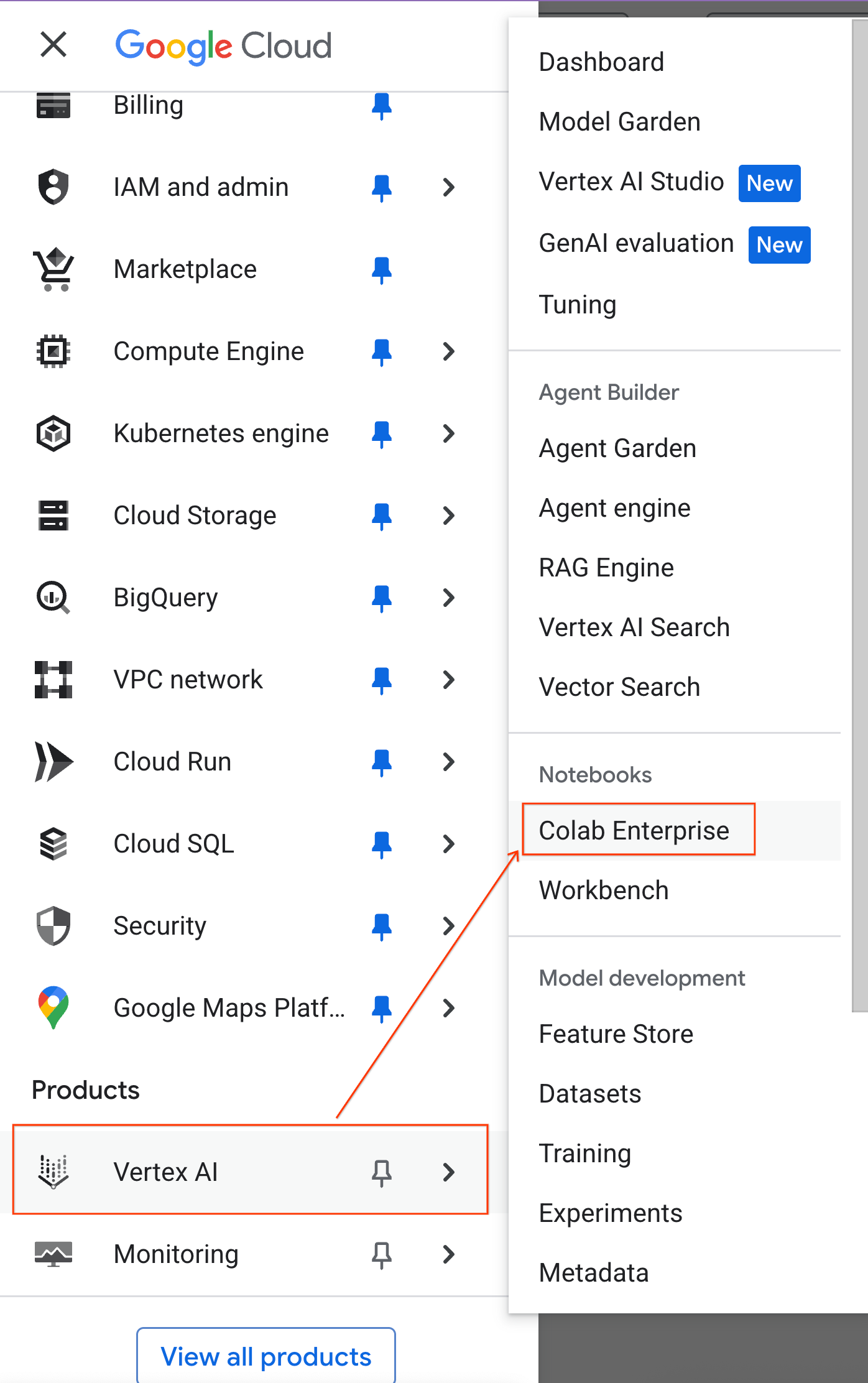
- 在 Google Cloud 控制台中,依次前往导航菜单 > Agent Platform > Notebooks。
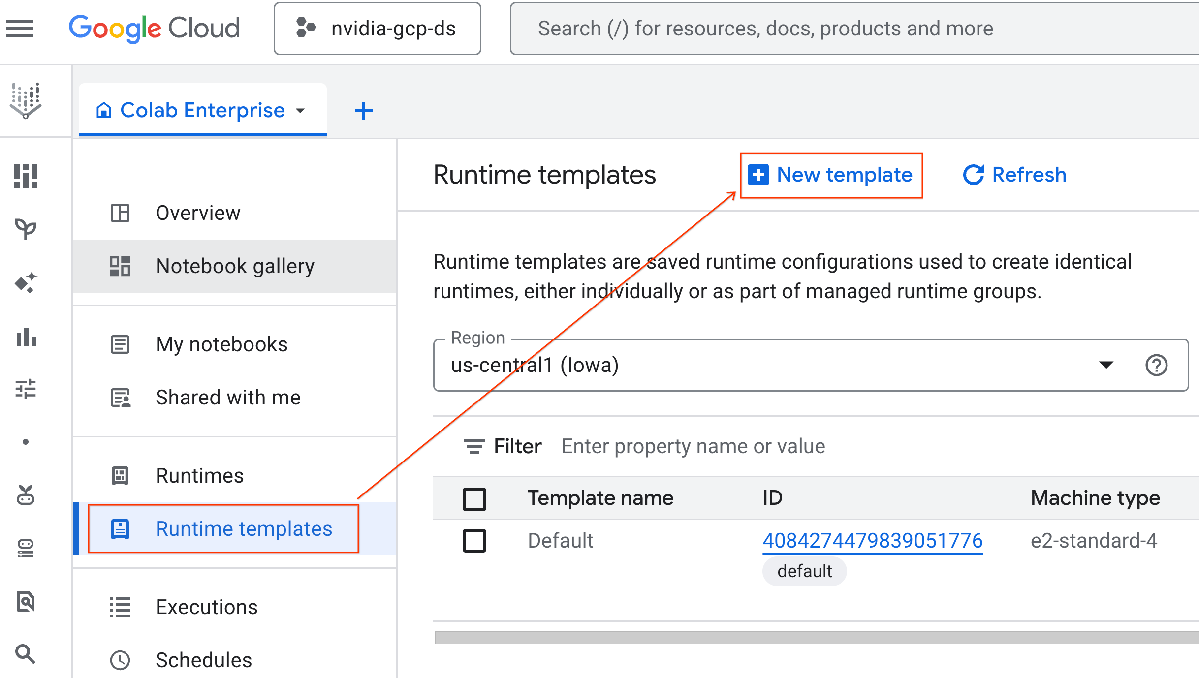
- 在 Colab Enterprise 中,点击运行时模板,然后选择新建模板。
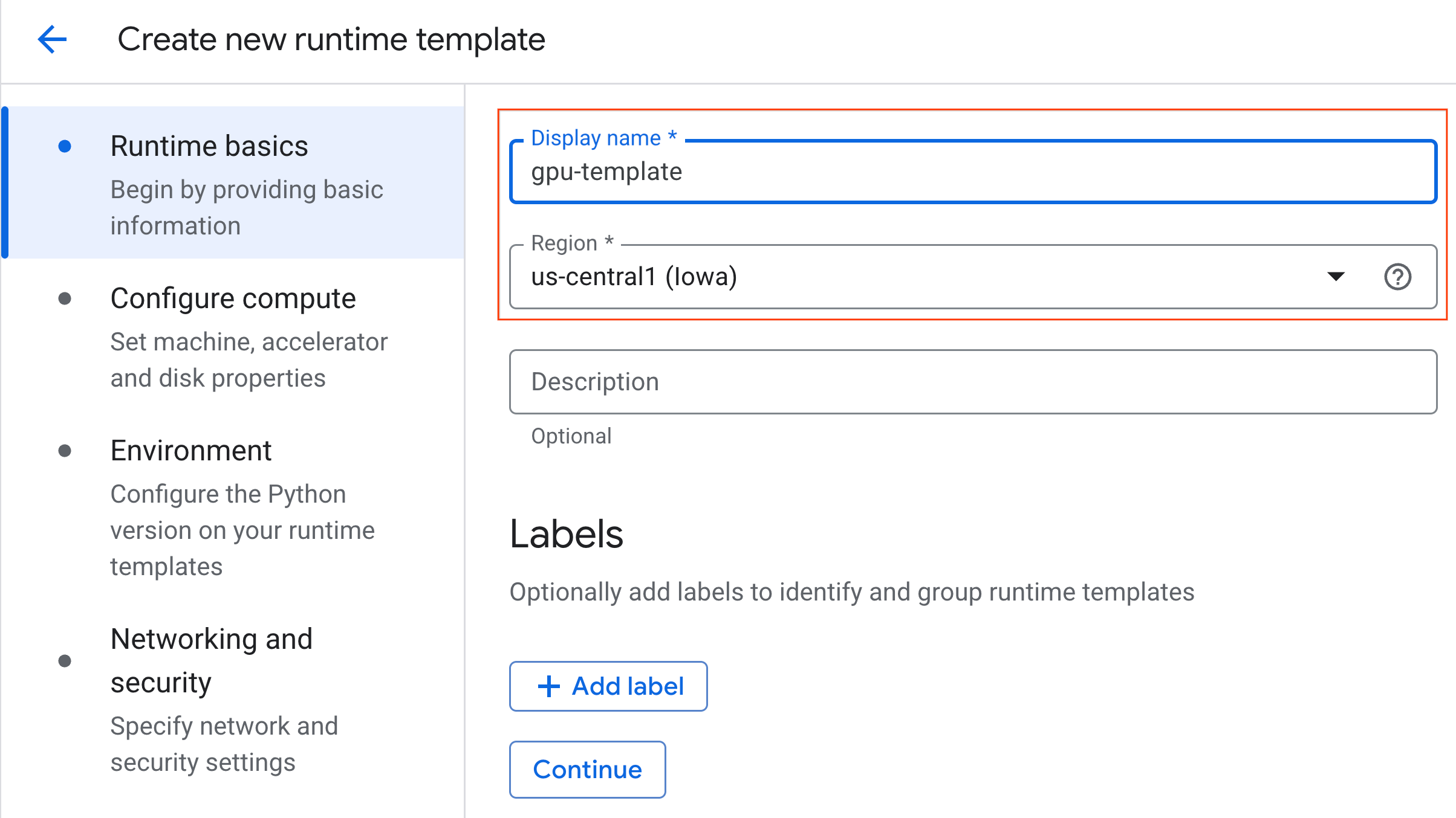
- 在运行时基本信息下:
- 将显示名称设置为
gpu-template。 - 设置您的首选区域。
- 将显示名称设置为
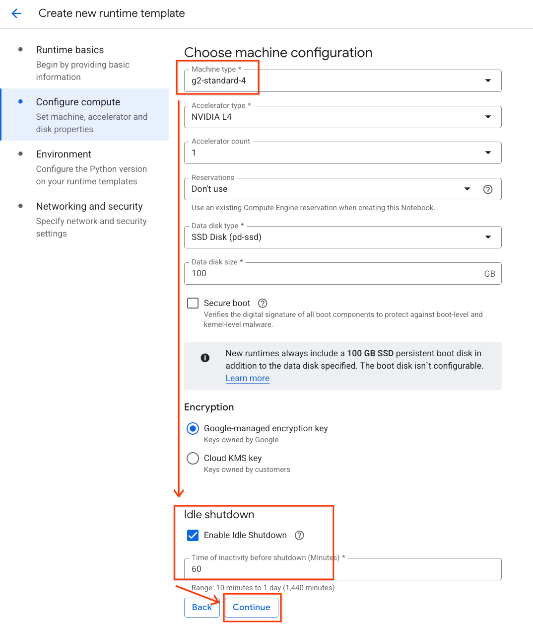
- 在配置计算下:
- 将机器类型设置为
g2-standard-4。 - 将默认加速器类型保留为
NVIDIA L4,并将加速器数量设置为 1。 - 将空闲关闭时间更改为 60 分钟。
- 点击继续。
- 将机器类型设置为
- 在环境下:
- 将环境设置为
Python 3.11
- 将环境设置为
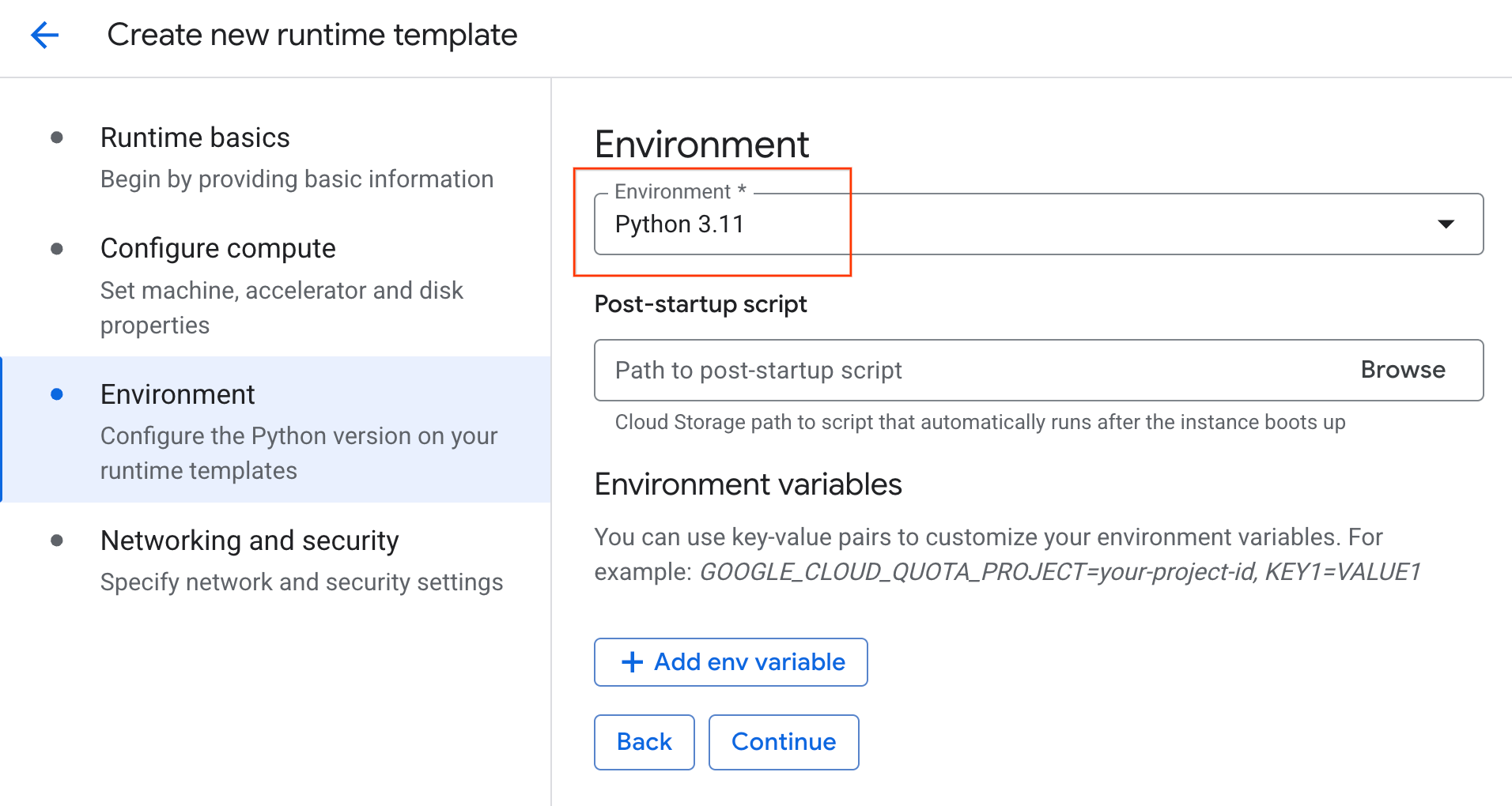
- 点击创建以保存运行时模板。您的“运行时模板”页面现在应会显示新模板。
6. 启动运行时
准备好模板后,您就可以创建新的运行时了。
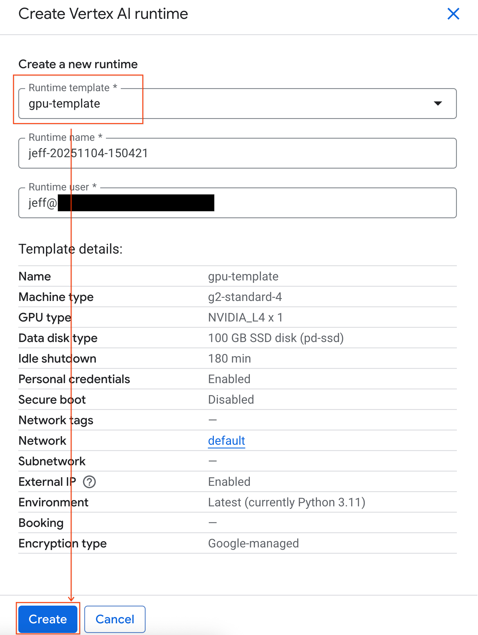
- 在 Colab Enterprise 中,点击运行时,然后选择创建。
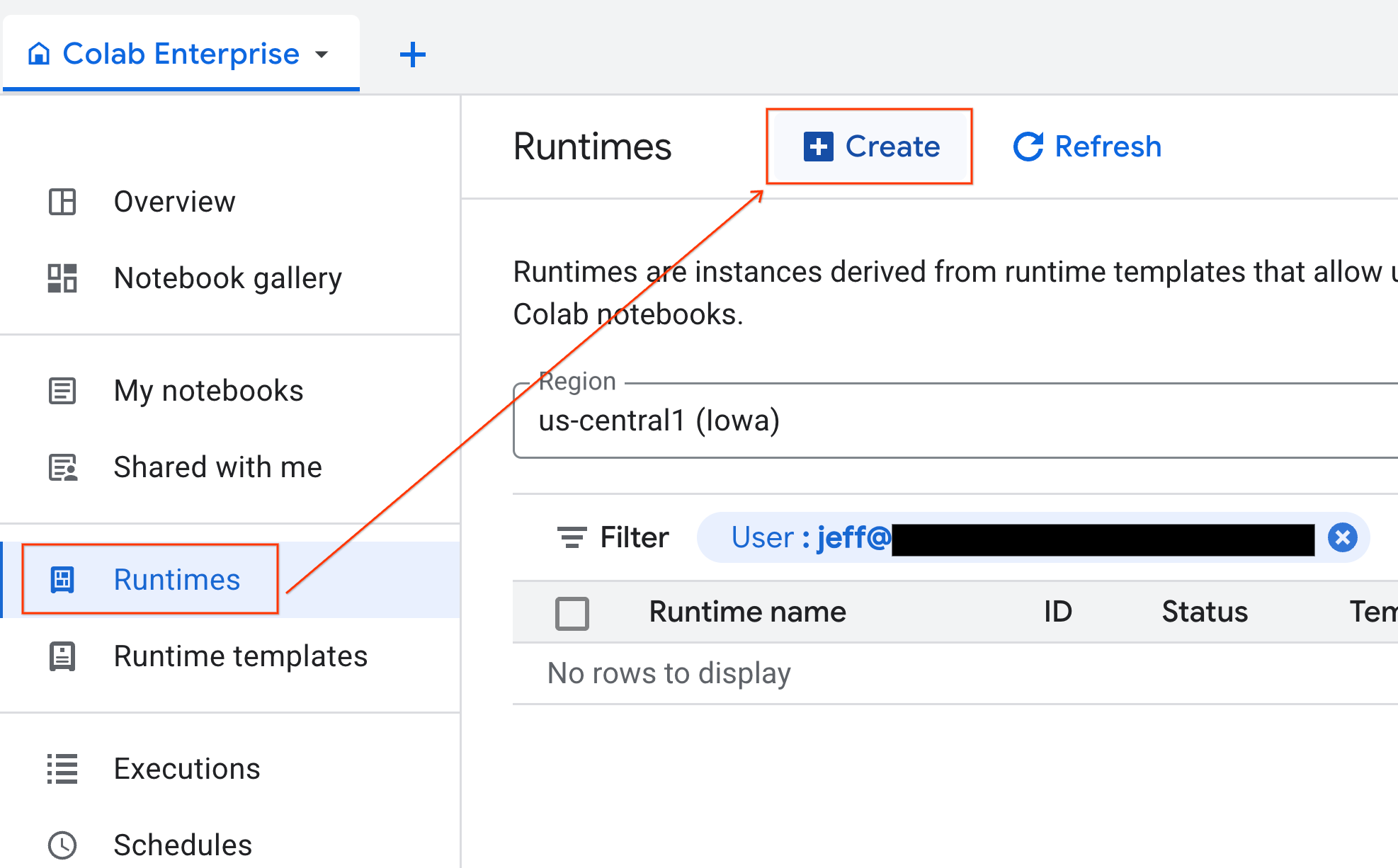
- 在运行时模板下方,选择
gpu-template选项。点击创建,然后等待运行时启动。
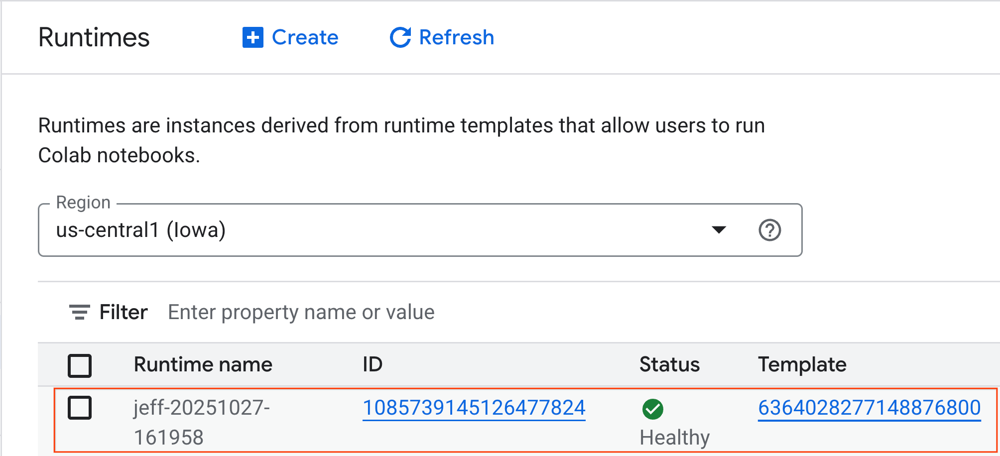
- 几分钟后,您会看到运行时可用。
7. 设置笔记本
现在,您的基础架构已在运行,您需要导入实验笔记本并将其连接到运行时。
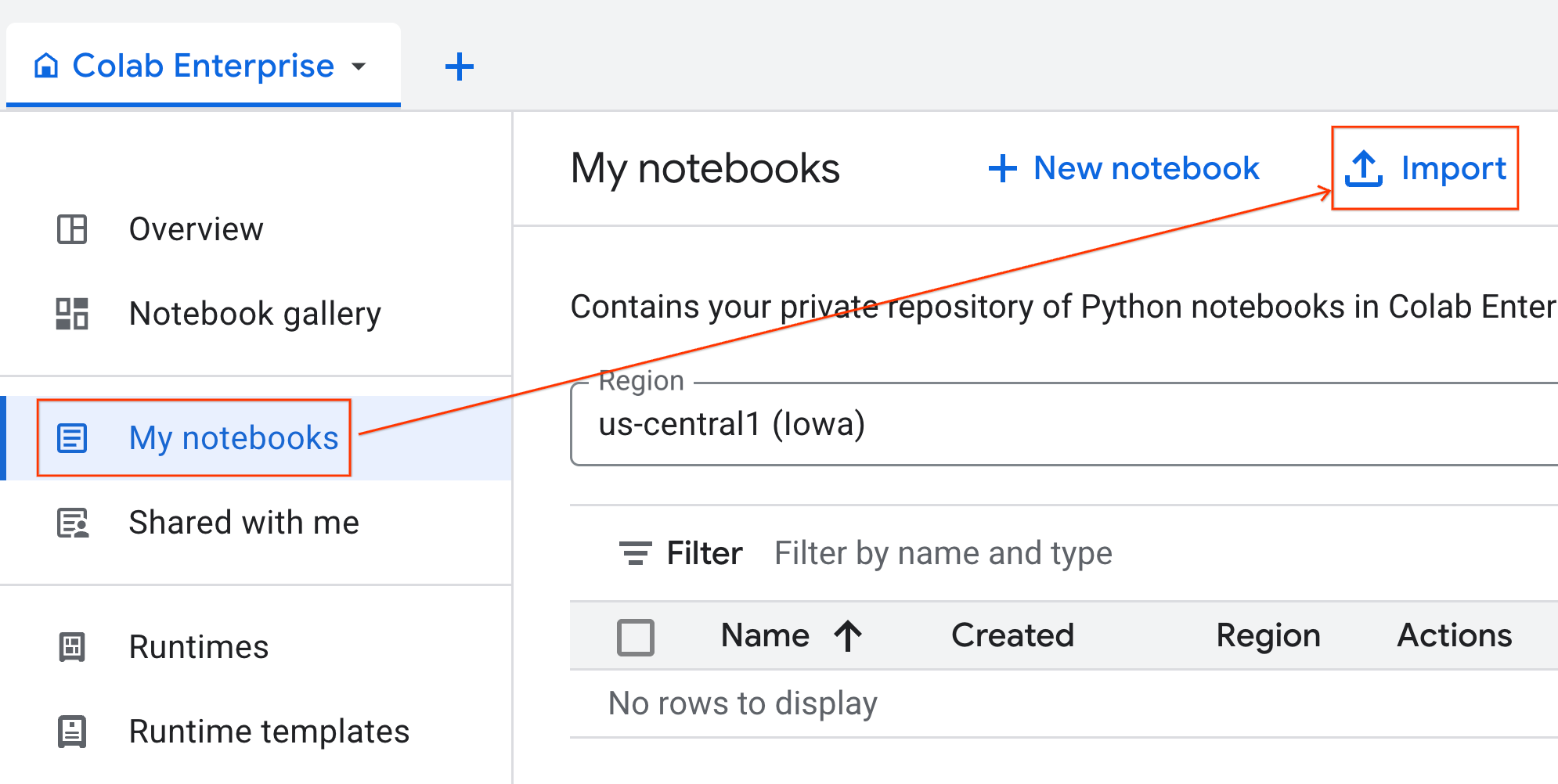
导入笔记本
- 在 Colab Enterprise 中,点击我的笔记本,然后点击导入。
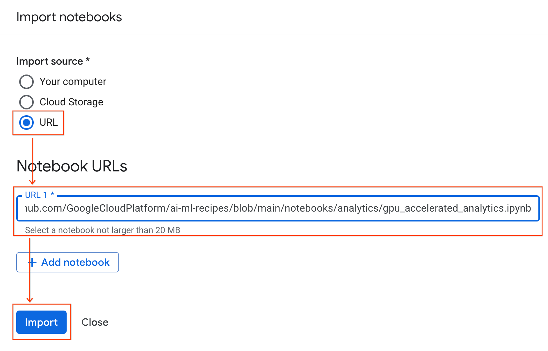
- 选择网址单选按钮,然后输入以下网址:
https://github.com/GoogleCloudPlatform/ai-ml-recipes/blob/main/notebooks/regression/gpu_accelerated_regression/gpu_accelerated_regression.ipynb
- 点击导入。Colab Enterprise 会将笔记本从 GitHub 复制到您的环境中。
连接到运行时
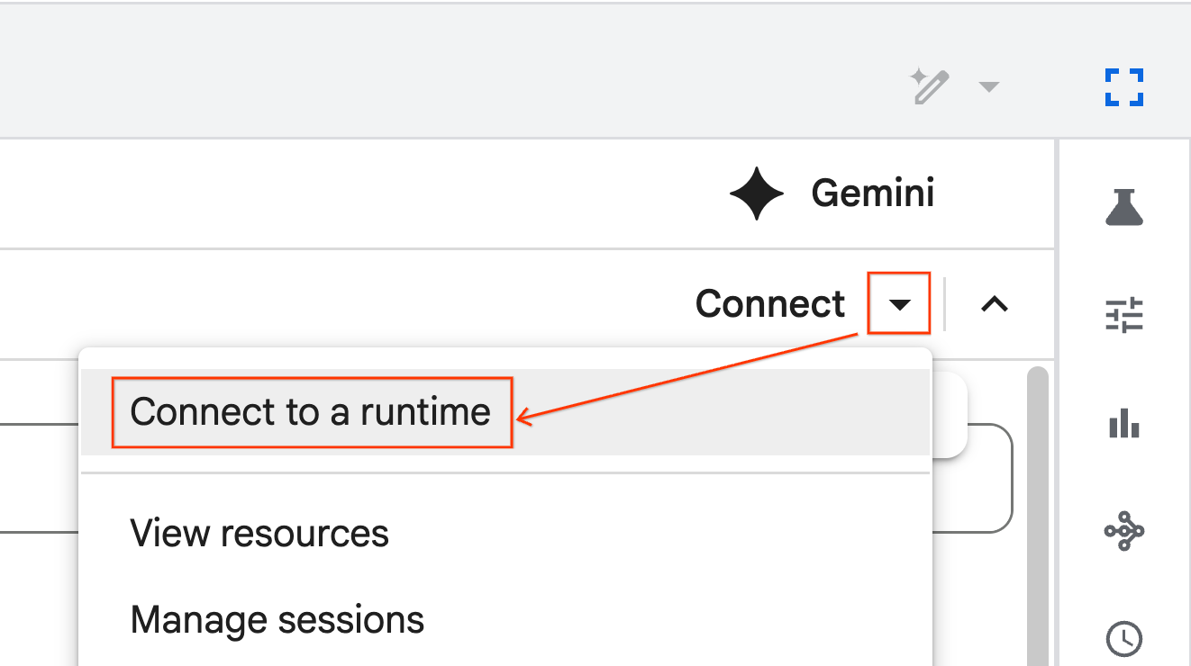
- 打开新导入的笔记本。
- 点击连接旁边的下拉箭头。
- 选择连接到运行时。
- 使用下拉菜单选择您之前创建的运行时。
- 点击连接。
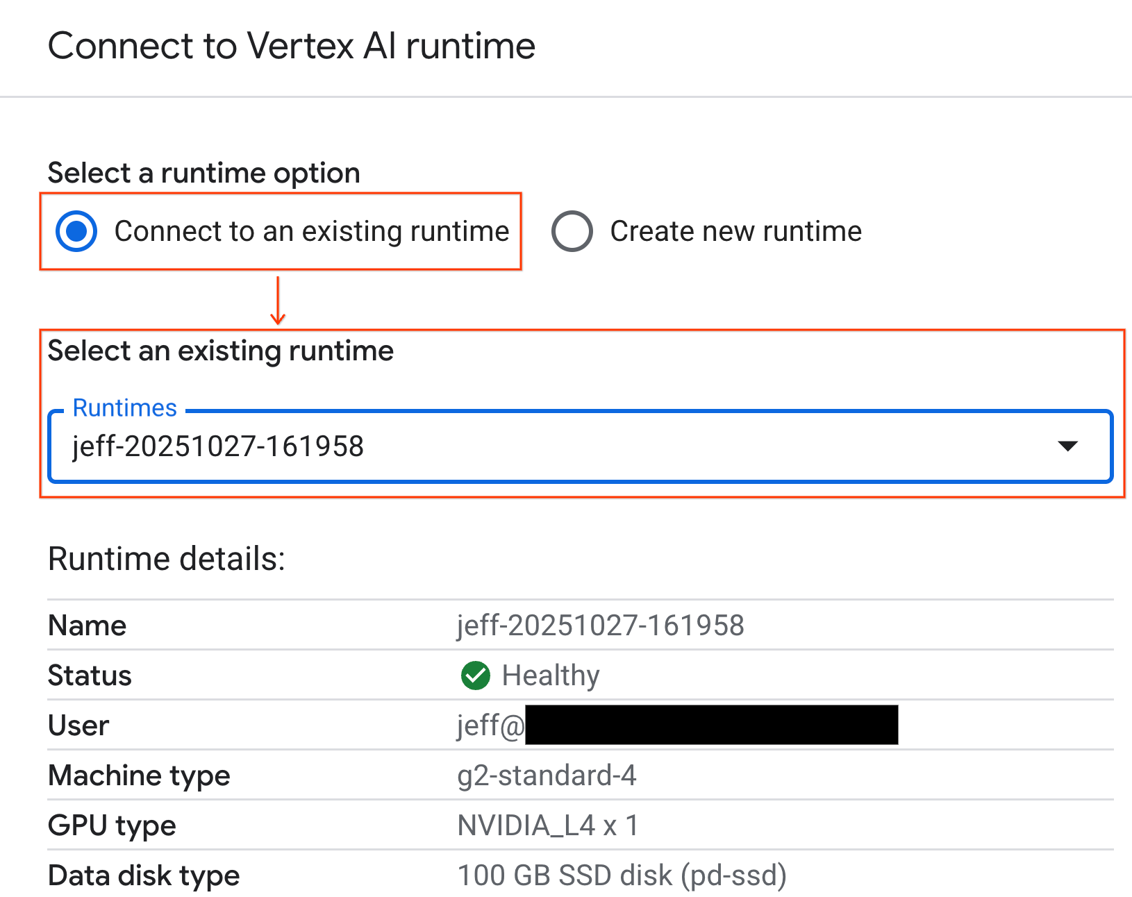
您的笔记本现已连接到启用 GPU 的运行时。
内置依赖项
使用 Colab Enterprise 的一个好处是,它预安装了您需要的库。对于本实验,您无需手动安装或管理 cuDF、cuML 或 XGBoost 等依赖项。
8. 准备纽约市出租车数据集
此 Codelab 使用 NYC Taxi & Limousine Commission (TLC) 行程记录数据。该数据集包含纽约市黄色出租车的行程记录,包括:
- 上车和下车日期、时间及地点
- 行程距离
- 分项车费金额
- 乘客人数
- 小费金额(这是我们将要预测的内容!)
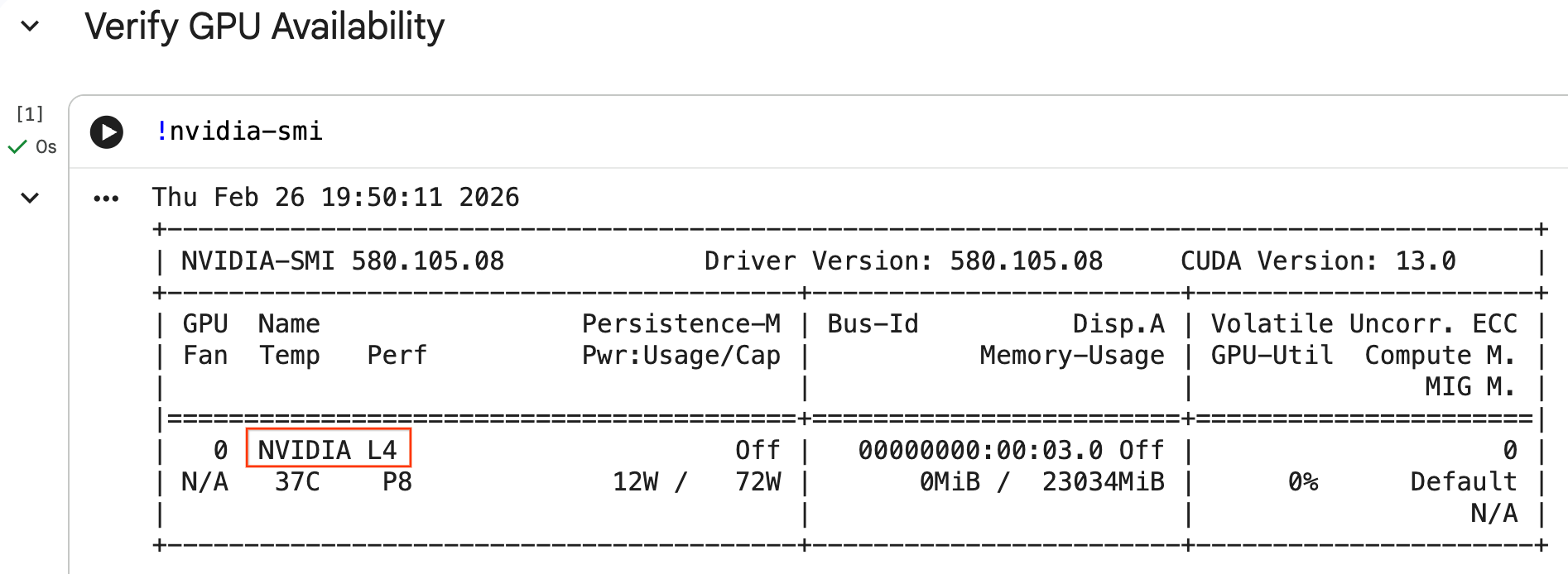
配置 GPU 并确认可用性
您可以运行 nvidia-smi 命令来确认 GPU 是否已被识别。它会显示驱动程序版本和 GPU 详细信息(例如 NVIDIA L4)。
nvidia-smi
该单元格应返回附加到运行时的 GPU,如下所示:
下载数据
下载 2024 年的行程数据。
from tqdm import tqdm
import requests
import time
import os

YEAR = 2024
DATA_DIR = "nyc_taxi_data"

os.makedirs(DATA_DIR, exist_ok=True)
print(f"Checking/Downloading files for {YEAR}...")

for month in tqdm(range(1, 13), unit="file"):
    file_name = f"yellow_tripdata_{YEAR}-{month:02d}.parquet"
    local_path = os.path.join(DATA_DIR, file_name)
    url = f"https://d37ci6vzurychx.cloudfront.net/trip-data/{file_name}"

    if not os.path.exists(local_path):
        try:
            with requests.get(url, stream=True) as response:
                response.raise_for_status()
                with open(local_path, 'wb') as f:
                    for chunk in response.iter_content(chunk_size=8192):
                        f.write(chunk)
            time.sleep(1)
        except requests.exceptions.HTTPError as e:
            print(f"\nSkipping {file_name}: {e}")
            if os.path.exists(local_path):
                os.remove(local_path)

print("\nDownload complete.")
借助 NVIDIA cuDF 加速 pandas
pandas 库在 CPU 上运行,处理大型数据集时速度可能会较慢。NVIDIA %load_ext cudf.pandas magic 命令会动态修补 pandas 以使用 GPU 加速,并在需要时回退到 CPU。
我们使用此 magic 命令,而不是标准导入,因为它可实现“零代码更改”加速。您无需重写任何现有代码。类似命令 %load_ext cuml.accel 可对 scikit-learn models 执行完全相同的操作!此功能适用于任何具有兼容 NVIDIA GPU 的 Jupyter 环境,而不仅仅是 Colab Enterprise。
%load_ext cudf.pandas
如需验证它是否处于活动状态,请导入 pandas 并检查其类型:
import pandas as pd

pd
输出将确认您现在使用的是 cudf.pandas 模块。
加载和清理数据
在 cudf.pandas 处于有效状态时,加载 Parquet 文件并执行数据清理。此过程会在 GPU 上自动运行。
import glob

# Load data into memory
df = pd.concat(
    [pd.read_parquet(f) for f in glob.glob("nyc_taxi_data/*-01.parquet")],
    ignore_index=True
)

# Filter for valid trips. We filter for payment_type=1 (credit card)
# because tip amounts are only reliably recorded for credit card transactions.
df = df[
    (df['fare_amount'] > 0) & (df['fare_amount'] < 500) &
    (df['trip_distance'] > 0) & (df['trip_distance'] < 100) &
    (df['tip_amount'] >= 0) & (df['tip_amount'] < 100) &
    (df['payment_type'] == 1)
].copy()

# Downcast numeric columns to save memory
float_cols = df.select_dtypes(include=['float64']).columns
df[float_cols] = df[float_cols].astype('float32')

int_cols = df.select_dtypes(include=['int64']).columns
df[int_cols] = df[int_cols].astype('int32')
特征工程
根据上车日期时间创建派生特征。该笔记本包含将在后续步骤中使用的其他功能。
import numpy as np

# Time Features
df['hour'] = df['tpep_pickup_datetime'].dt.hour
df['dow'] = df['tpep_pickup_datetime'].dt.dayofweek
df['is_weekend'] = (df['dow'] >= 5).astype(int)
df['is_rush_hour'] = (
    ((df['hour'] >= 7) & (df['hour'] <= 9)) |
    ((df['hour'] >= 17) & (df['hour'] <= 19))
).astype(int)

...
# Other features
...
9. 使用交叉验证训练单个模型
为了展示 GPU 如何加速机器学习,您将训练三种不同的回归模型来预测出租车行程的 tip_amount。
借助 NVIDIA cuML 加速 scikit-learn
使用 NVIDIA cuML 在 GPU 上运行 scikit-learn 算法,而无需更改 API 调用。首先,加载 cuml.accel 扩展程序。
%load_ext cuml.accel
设置功能和目标
确定您希望模型学习的特征,并拆分出目标列 (tip_amount)。
feature_cols = [
    'trip_distance', 'fare_amount', 'passenger_count',
    'hour', 'dow', 'is_weekend', 'is_rush_hour',
    'fare_log', 'fare_decimal', 'is_round_fare',
    'route_frequency', 'pu_tip_mean', 'pu_tip_std',
    'PULocationID', 'DOLocationID'
]

X = df[feature_cols].fillna(df[feature_cols].median())
y = df['tip_amount'].copy()
设置交叉验证拆分,以稳健地评估模型性能。
from sklearn.model_selection import KFold
import numpy as np
import time
from sklearn.metrics import mean_squared_error
from tqdm.notebook import tqdm

n_splits = 3
kf = KFold(n_splits=n_splits, shuffle=True, random_state=42)
1. XGBoost
XGBoost 本身就支持 GPU 加速。传递 tree_method='hist' 和 device='cuda' 以在训练期间使用 GPU。
import xgboost as xgb

start_time = time.perf_counter()

def train_xgb_cv(X, y):
    rmses = []
    preds_all = np.zeros(len(y))
    for train_idx, val_idx in tqdm(kf.split(X), total=n_splits):
        X_train, X_val = X.iloc[train_idx], X.iloc[val_idx]
        y_train, y_val = y.iloc[train_idx], y.iloc[val_idx]

        # XGBoost handles GPU natively when tree_method='hist' and device='cuda'
        model = xgb.XGBRegressor(
            objective='reg:squarederror',
            max_depth=5,
            learning_rate=0.1,
            n_estimators=100,
            tree_method='hist',
            device='cuda',
            random_state=42
        )
        model.fit(X_train, y_train)

        preds = model.predict(X_val)
        preds_all[val_idx] = preds
        rmses.append(np.sqrt(mean_squared_error(y_val, preds)))

    return np.mean(rmses), preds_all

xgb_rmse, xgb_preds = train_xgb_cv(X, y)
print(f"\n{'XGBoost RMSE:':<20} ${xgb_rmse:.4f}")
print(f"{'Time:':<20} {time.perf_counter() - start_time:.2f} seconds")
2. 线性回归
训练线性回归模型。在 %load_ext cuml.accel 处于有效状态时,LinearRegression 会自动映射到其 GPU 等效项。
from sklearn.linear_model import LinearRegression
from sklearn.preprocessing import StandardScaler

start_time = time.perf_counter()

def train_linreg_cv(X, y):
    rmses = []
    preds_all = np.zeros(len(y))
    for train_idx, val_idx in tqdm(kf.split(X), total=n_splits):
        X_train, X_val = X.iloc[train_idx], X.iloc[val_idx]
        y_train, y_val = y.iloc[train_idx], y.iloc[val_idx]

        # Scale features
        scaler = StandardScaler()
        X_train_scaled = scaler.fit_transform(X_train)
        X_val_scaled = scaler.transform(X_val)

        # Automatically accelerated by cuML
        model = LinearRegression()
        model.fit(X_train_scaled, y_train)

        preds = model.predict(X_val_scaled)
        preds_all[val_idx] = preds
        rmses.append(np.sqrt(mean_squared_error(y_val, preds)))

    return np.mean(rmses), preds_all

linreg_rmse, linreg_preds = train_linreg_cv(X, y)
print(f"\n{'Linear Reg RMSE:':<20} ${linreg_rmse:.4f}")
print(f"{'Time:':<20} {time.perf_counter() - start_time:.2f} seconds")
3. 随机森林
使用 RandomForestRegressor 训练集成模型。基于树的模型在 CPU 上训练时通常速度较慢,但 GPU 加速可更快地处理数百万行数据。
from sklearn.ensemble import RandomForestRegressor

start_time = time.perf_counter()

def train_rf_cv(X, y):
    rmses = []
    preds_all = np.zeros(len(y))
    for train_idx, val_idx in tqdm(kf.split(X), total=n_splits):
        X_train, X_val = X.iloc[train_idx], X.iloc[val_idx]
        y_train, y_val = y.iloc[train_idx], y.iloc[val_idx]

        # Automatically accelerated by cuML
        model = RandomForestRegressor(
            n_estimators=100,
            max_depth=10,
            n_jobs=-1,
            max_features='sqrt',
            random_state=42
        )
        model.fit(X_train, y_train)

        preds = model.predict(X_val)
        preds_all[val_idx] = preds
        rmses.append(np.sqrt(mean_squared_error(y_val, preds)))

    return np.mean(rmses), preds_all

rf_rmse, rf_preds = train_rf_cv(X, y)
print(f"\n{'Random Forest RMSE:':<20} ${rf_rmse:.4f}")
print(f"{'Time:':<20} {time.perf_counter() - start_time:.2f} seconds")
10. 评估端到端流水线
使用简单的线性集成模型组合这三个模型的预测结果。与单个模型相比,这种方法通常可略微提高准确率。
对预测结果拟合线性回归,以找到最佳权重:
ensemble_weights = LinearRegression(positive=True, fit_intercept=False).fit(
    np.c_[xgb_preds, rf_preds, linreg_preds], y
).coef_

# Normalize weights
ensemble_weights = ensemble_weights / ensemble_weights.sum()

ensemble_preds = np.c_[xgb_preds, rf_preds, linreg_preds] @ ensemble_weights
ensemble_rmse = np.sqrt(mean_squared_error(y, ensemble_preds))
比较结果,查看集成学习的提升效果:
print(f"\n{'Model':<20} {'RMSE':>10}")
print("-" * 32)
print(f"{'Linear Regression':<20} ${linreg_rmse:>9.4f}")
print(f"{'Random Forest':<20} ${rf_rmse:>9.4f}")
print(f"{'XGBoost':<20} ${xgb_rmse:>9.4f}")
print("-" * 32)
print(f"{'Ensemble':<20} ${ensemble_rmse:>9.4f}")
print(f"\nEnsemble lift: ${xgb_rmse - ensemble_rmse:.4f}")
11. 比较 CPU 与 GPU 的性能
为了正确衡量性能差异,您将重启内核以确保执行状态干净,在 CPU 上运行整个数据科学流水线,然后在 GPU 上再次运行该流水线。
重启内核
运行 IPython.Application.instance().kernel.do_shutdown(True) 命令以重启内核并释放内存。
import IPython
IPython.Application.instance().kernel.do_shutdown(True)
定义数据科学流水线
将核心工作流(加载数据、清理、特征工程和模型训练)封装到单个函数中。此函数接受 pandas 模块 pd_module 和 use_gpu 实参,以在环境之间切换。
def run_ml_pipeline(pd_module, use_gpu=False):
    import time
    import glob
    import numpy as np
    from sklearn.ensemble import RandomForestRegressor
    import xgboost as xgb

    timings = {}

    # 1. Load Data
    t0 = time.perf_counter()
    df = pd_module.concat(
        [pd_module.read_parquet(f) for f in glob.glob("nyc_taxi_data/*-01.parquet")],
        ignore_index=True
    )
    timings['Load Data'] = time.perf_counter() - t0

    # 2. Clean Data
    t0 = time.perf_counter()
    # Filter for payment_type=1 (credit card) because tip amounts
    # are only reliably recorded for credit card transactions.
    df = df[
        (df['fare_amount'] > 0) & (df['fare_amount'] < 500) &
        (df['trip_distance'] > 0) & (df['trip_distance'] < 100) &
        (df['tip_amount'] >= 0) & (df['tip_amount'] < 100) &
        (df['payment_type'] == 1)
    ].copy()

    # Downcast numeric columns to save memory
    float_cols = df.select_dtypes(include=['float64']).columns
    df[float_cols] = df[float_cols].astype('float32')
    int_cols = df.select_dtypes(include=['int64']).columns
    df[int_cols] = df[int_cols].astype('int32')
    timings['Clean Data'] = time.perf_counter() - t0

    # 3. Feature Engineering
    t0 = time.perf_counter()
    df['hour'] = df['tpep_pickup_datetime'].dt.hour
    df['dow'] = df['tpep_pickup_datetime'].dt.dayofweek
    df['is_weekend'] = (df['dow'] >= 5).astype(int)
    df['fare_log'] = np.log1p(df['fare_amount'])
    timings['Feature Engineering'] = time.perf_counter() - t0

    # 4. Modeling Prep
    feature_cols = ['trip_distance', 'fare_amount', 'passenger_count', 'hour', 'dow', 'is_weekend', 'fare_log']
    X = df[feature_cols].fillna(df[feature_cols].median())
    y = df['tip_amount'].copy()

    # Free memory
    del df
    import gc
    gc.collect()

    # 5. Train Random Forest
    t0 = time.perf_counter()
    rf_model = RandomForestRegressor(
        n_estimators=100,
        max_depth=10,
        n_jobs=-1,
        max_features='sqrt',
        random_state=42
    ).fit(X, y)
    timings['Train Random Forest'] = time.perf_counter() - t0

    # 6. Train XGBoost
    t0 = time.perf_counter()
    params = {
        'objective': 'reg:squarederror',
        'max_depth': 5,
        'n_estimators': 100,
        'random_state': 42
    }
    if use_gpu:
        params['device'] = 'cuda'
        params['tree_method'] = 'hist'
    xgb_model = xgb.XGBRegressor(**params).fit(X, y)
    timings['Train XGBoost'] = time.perf_counter() - t0

    del X
    del y
    gc.collect()

    return timings
在 CPU 上运行
使用标准 CPU pandas 调用流水线。
import pandas as pd

print("Running pipeline on CPU...")
cpu_times = run_ml_pipeline(pd, use_gpu=False)
print("CPU Execution Finished.")
在 GPU 上运行
加载 NVIDIA 库扩展程序,将加速的 cudf.pandas 模块传递给流水线,并在内部将 XGBoost 设备设置为 cuda。
import IPython.core.magic
if not hasattr(IPython.core.magic, 'output_can_be_silenced'):
    IPython.core.magic.output_can_be_silenced = lambda x: x

%load_ext cudf.pandas
%load_ext cuml.accel
import pandas as pd

print("Running pipeline on GPU...")
gpu_times = run_ml_pipeline(pd, use_gpu=True)
print("GPU Execution Finished.")
直观呈现性能加速效果
使用 matplotlib 可视化时间。结果显示了使用 GPU 时在数据处理和模型训练期间节省的时间。
import matplotlib.pyplot as plt
import numpy as np

labels = list(cpu_times.keys())
cpu_values = list(cpu_times.values())
gpu_values = list(gpu_times.values())

x = np.arange(len(labels))
width = 0.35

fig, ax = plt.subplots(figsize=(10, 6))
rects1 = ax.bar(x - width/2, cpu_values, width, label='CPU', color='#4285F4')
rects2 = ax.bar(x + width/2, gpu_values, width, label='GPU', color='#76B900')

ax.set_ylabel('Execution Time (seconds)')
ax.set_title('NYC Taxi ML Pipeline: CPU vs. GPU Performance')
ax.set_xticks(x)
ax.set_xticklabels(labels, rotation=45, ha="right")
ax.legend()

# Add data labels
def autolabel(rects):
    for rect in rects:
        height = rect.get_height()
        ax.annotate(f'{height:.2f}s',
                    xy=(rect.get_x() + rect.get_width() / 2, height),
                    xytext=(0, 3),  # 3 points vertical offset
                    textcoords="offset points",
                    ha='center', va='bottom', fontsize=9)
autolabel(rects1)
autolabel(rects2)

plt.tight_layout()
plt.show()

# Calculate overall speedup
total_cpu_time = sum(cpu_values)
total_gpu_time = sum(gpu_values)
overall_speedup = total_cpu_time / total_gpu_time
print(f"\nOverall Pipeline Speedup: {overall_speedup:.2f}x faster on GPU!")
您应该会看到类似如下内容:
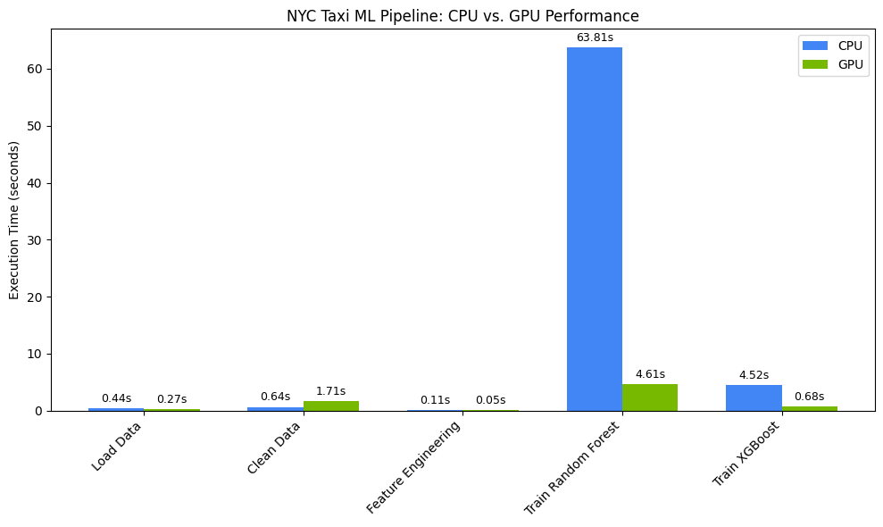
此图表展示了 GPU 在整个数据科学工作流程中的显著性能优势。对于随机森林和 XGBoost 等算法,您应该会在计算密集型模型训练阶段看到最显著的节省时间效果。
12. 分析代码以找出性能限制
使用 cudf.pandas 时,大多数函数都在 GPU 上运行。如果 cuDF 尚不支持特定操作,执行会暂时回退到 CPU。NVIDIA 提供了两个内置的 Jupyter 魔法命令来识别这些回退。
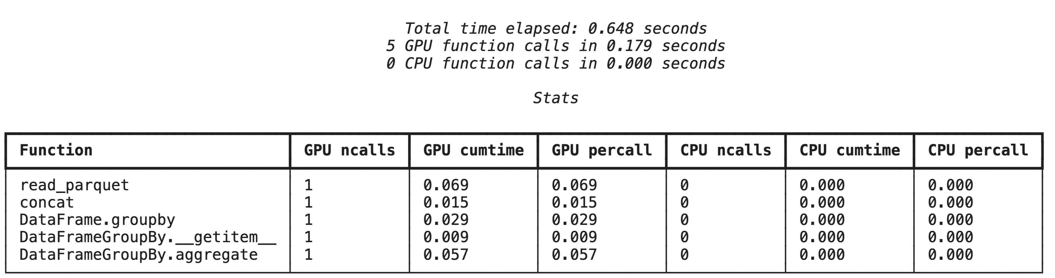
使用 %%cudf.pandas.profile 进行高级别分析
%%cudf.pandas.profile magic 命令可提供在 GPU 或 CPU 上运行的函数的摘要。
%%cudf.pandas.profile

import glob
import pandas as pd

df = pd.concat([pd.read_parquet(f) for f in glob.glob("nyc_taxi_data/*-01.parquet")], ignore_index=True)

summary = (
    df
      .groupby(['PULocationID', 'payment_type'])
      [['passenger_count', 'fare_amount', 'tip_amount']]
      .agg(['min', 'mean', 'max'])
)
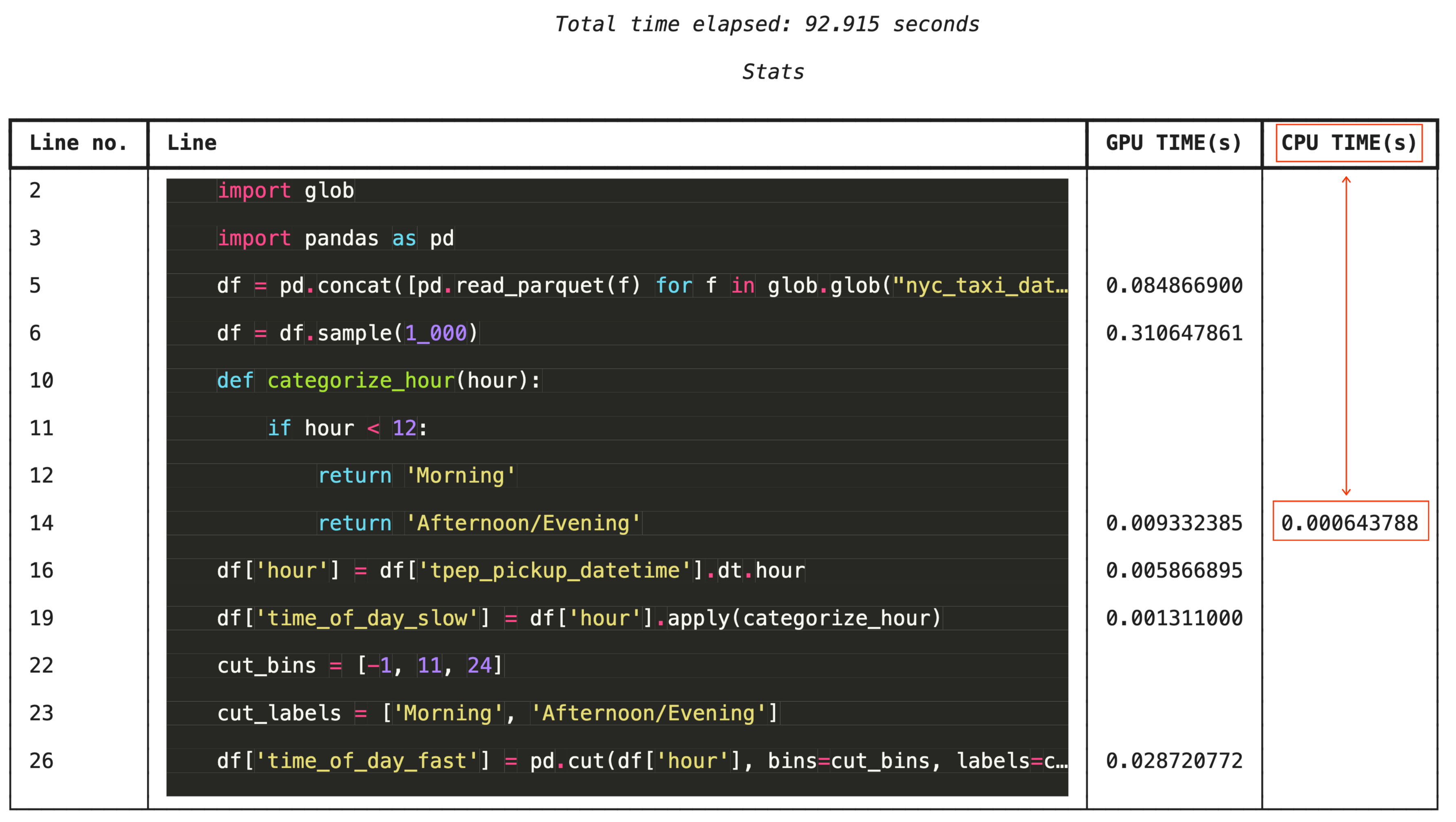
使用 %%cudf.pandas.line_profile 进行逐行分析
为了进行精细的问题排查,%%cudf.pandas.line_profile 会在每行代码中添加注释,说明该代码在 GPU 上和 CPU 上执行的次数。
%%cudf.pandas.line_profile

import glob
import pandas as pd

df = pd.concat([pd.read_parquet(f) for f in glob.glob("nyc_taxi_data/*-01.parquet")], ignore_index=True)
df = df.sample(1_000)

# Iterating row-by-row or using custom python apply functions often falls back to the CPU
def categorize_hour(hour):
    if hour < 12:
        return 'Morning'
    else:
        return 'Afternoon/Evening'

df['hour'] = df['tpep_pickup_datetime'].dt.hour

df['time_of_day_slow'] = df['hour'].apply(categorize_hour)

# Using vectorized pandas operations (like pd.cut) stays entirely on the GPU
cut_bins = [-1, 11, 24]
cut_labels = ['Morning', 'Afternoon/Evening']
df['time_of_day_fast'] = pd.cut(df['hour'], bins=cut_bins, labels=cut_labels)
13. 清理
为避免您的 Google Cloud 账号产生意外费用,请清理您在此 Codelab 期间创建的资源。
删除资源
在笔记本单元格中使用 !rm -rf 命令删除运行时中的本地数据集。
print("Deleting local 'nyc_taxi_data' directory...")
!rm -rf nyc_taxi_data
print("Local files deleted.")
关闭 Colab 运行时
- 在 Google Cloud 控制台中,前往 Colab Enterprise 运行时页面。
- 在区域菜单中,选择包含运行时的区域。
- 选择要删除的运行时。
- 点击删除。
- 点击确认。
删除笔记本
- 在 Google Cloud 控制台中,前往 Colab Enterprise 我的笔记本页面。
- 在区域菜单中,选择包含笔记本的区域。
- 选择要删除的笔记本。
- 点击删除。
- 点击确认。
14. 恭喜
恭喜!您已成功在 Colab Enterprise 上使用 NVIDIA cuDF 和 cuML 库加速了 pandas 和 scikit-learn 机器学习工作流。只需添加几个 magic 命令(%load_ext cudf.pandas 和 %load_ext cuml.accel),您的标准代码即可在 GPU 上运行,从而在极短的时间内处理记录并在本地拟合复杂模型。
如需详细了解如何使用 GPU 加速数据分析,请参阅 Accelerated Data Analytics with GPUs (使用 GPU 加速数据分析) Codelab。
所学内容
- 了解 Google Cloud 上的 Colab Enterprise。
- 使用特定的 GPU 和内存配置自定义 Colab 运行时环境。
- 应用 GPU 加速功能,使用纽约市出租车数据集中的数百万条记录预测小费金额。
- 使用 NVIDIA 的
cuDF库,在不更改任何代码的情况下加速pandas。 - 使用 NVIDIA 的
cuML库和 GPU,无需更改任何代码即可加速scikit-learn。 - 分析代码以找出并优化性能限制。