
1. 簡介
在本程式碼研究室中,您將瞭解如何使用 Google Cloud 上的 NVIDIA GPU 和開放原始碼程式庫,加快處理大型資料集的資料科學和機器學習工作流程。首先,您將設定基礎架構,然後瞭解如何套用 GPU 加速功能。
您將著重於資料科學生命週期,從使用 pandas 準備資料,到使用 scikit-learn 和 XGBoost 訓練模型。您將瞭解如何使用 NVIDIA 的 cuDF 和 cuML 程式庫加速執行這些工作。最棒的是,您不必變更現有的 pandas 或 scikit-learn 程式碼,就能取得這項 GPU 加速功能。
課程內容
- 瞭解 Google Cloud 上的 Colab Enterprise。
- 自訂 Colab 執行階段環境,設定特定 GPU 和記憶體。
- 運用 GPU 加速功能,使用紐約市計程車資料集中的數百萬筆記錄,預測小費金額。
- 使用 NVIDIA 的
cuDF程式庫,在完全不修改程式碼的情況下加速pandas。 - 使用 NVIDIA 的
cuML程式庫和 GPU,無需變更任何程式碼即可加速scikit-learn。 - 分析程式碼,找出並改善效能限制。
下一頁會顯示可用於完成實驗室的抵免額。
2. 為什麼要加速機器學習?
機器學習需要加快疊代速度
準備資料相當耗時,隨著資料集變大,模型訓練或評估可能需要更長時間。使用 CPU 訓練隨機森林或 XGBoost 等模型,處理數百萬列資料可能需要數小時或數天。
使用 GPU 可透過 cuML 和 GPU 加速的 XGBoost 等程式庫,加快這些訓練執行作業的速度。這項加速功能可讓您:
- 加快疊代速度:快速測試新功能和超參數。
- 使用完整資料集進行訓練:請使用完整資料,而非經過降採樣的資料,以提高準確度。
- 降低費用:在更短的時間內完成大量工作負載,進而降低運算費用。
3. 設定和需求條件
潛在費用
本程式碼實驗室會使用 Google Cloud 資源,包括搭載 NVIDIA L4 GPU 的 Colab Enterprise 執行階段。請注意可能產生的費用,並按照程式碼研究室結尾的「清除」Clean Up一節操作,關閉資源並避免持續計費。如需詳細的定價資訊,請參閱 Colab Enterprise 定價和 GPU 定價。
事前準備
我們假設您已具備中等程度的 Python、pandas、scikit-learn 和標準機器學習實務 (例如交叉驗證/整合) 知識。
- 在 Google Cloud 控制台的專案選取器頁面中,選取或建立 Google Cloud 專案。
- 請確認 Google Cloud 專案已啟用計費功能。
啟用 API
如要使用 Colab Enterprise,請先啟用必要的 API。
- 點選 Google Cloud 控制台右上角的 Cloud Shell 圖示,開啟 Google Cloud Shell。

- 在 Cloud Shell 中,將
PROJECT_ID替換為您的專案 ID,設定專案 ID:
gcloud config set project <PROJECT_ID>
- 執行下列指令,啟用必要 API:
gcloud services enable \
    compute.googleapis.com \
    dataform.googleapis.com \
    notebooks.googleapis.com \
    aiplatform.googleapis.com
執行成功後,您應該會看到類似下方的訊息:
Operation "operations/..." finished successfully.
4. 選擇筆記本環境
許多資料科學家都熟悉 Colab,並將其用於個人專案,但 Colab Enterprise 提供安全、協作式且整合的筆記本體驗,專為企業設計。
在 Google Cloud 中,您有兩個主要的代管筆記本環境選項:Colab Enterprise 和 Gemini Enterprise Agent Platform Workbench。選擇哪種服務取決於專案的優先順序。
Agent Platform Workbench 的使用時機
如果優先考量控制和深度自訂,請選擇 Agent Platform Workbench。如果您需要執行下列操作,這就是理想的選擇:
- 管理基礎架構和機器生命週期。
- 使用自訂容器和網路設定。
- 與 MLOps 管道和自訂生命週期工具整合。
使用 Colab Enterprise 的時機
如果您的首要考量是快速設定、簡單易用和安全協作,請選擇 Colab Enterprise。這項全代管解決方案可讓團隊專心進行分析,不必費心處理基礎架構。
Colab Enterprise 可協助您:
- 開發與資料倉儲密切相關的資料科學工作流程。您可以直接在 BigQuery Studio 中開啟及管理筆記本。
- 訓練機器學習模型,並在 Agent Platform 中與 MLOps 工具整合。
- 享受彈性且統一的體驗。在 BigQuery 中建立的 Colab Enterprise 筆記本,可以在 Agent Platform 中開啟及執行,反之亦然。
今天的實驗室
本程式碼研究室使用 Colab Enterprise 加速機器學習。
如要進一步瞭解兩者的差異,請參閱選擇合適的 Notebook 解決方案官方說明文件。
5. 設定執行階段範本
在 Colab Enterprise 中,連線至以預先設定的執行階段範本為基礎的執行階段。
執行階段範本是可重複使用的設定,可指定筆記本的環境,包括:
- 機型 (CPU、記憶體)
- 加速器 (GPU 類型和數量)
- 磁碟大小和類型
- 聯播網設定和安全性政策
- 自動閒置關機規則
執行階段範本的優點
- 一致性:您和團隊可使用相同的環境,確保工作可重複執行。
- 安全性:範本會強制執行機構安全性政策。
- 成本管理:範本中已預先設定資源大小,有助於避免產生意外費用。
建立執行階段範本
為實驗室設定可重複使用的執行階段範本。
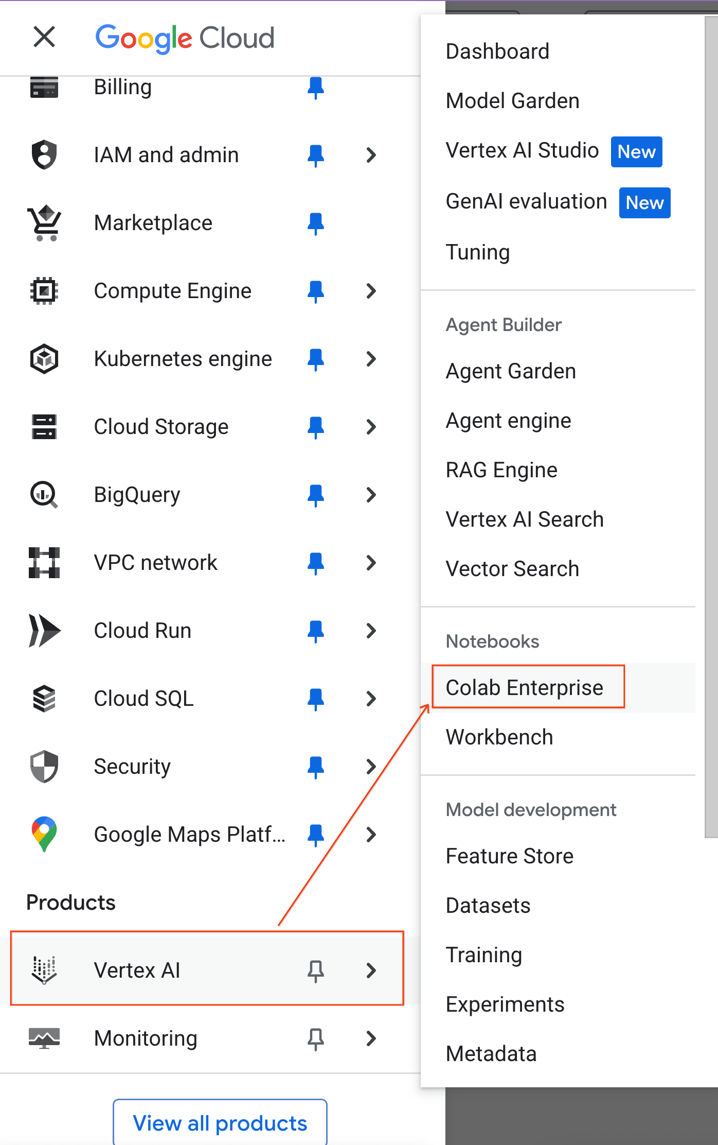
- 在 Google Cloud 控制台中,依序前往「導覽選單」 >「Agent Platform」 >「Notebooks」。
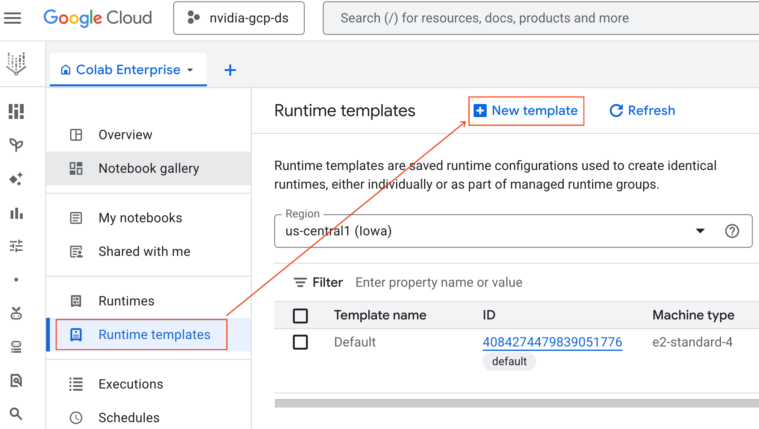
- 在 Colab Enterprise 中,按一下「執行階段範本」,然後選取「新增範本」。
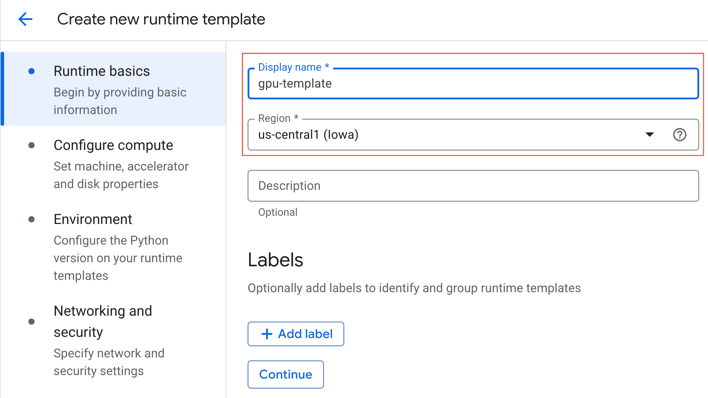
- 在「執行階段基本概念」下方:
- 將「顯示名稱」設為
gpu-template。 - 設定偏好的「地區」。
- 將「顯示名稱」設為
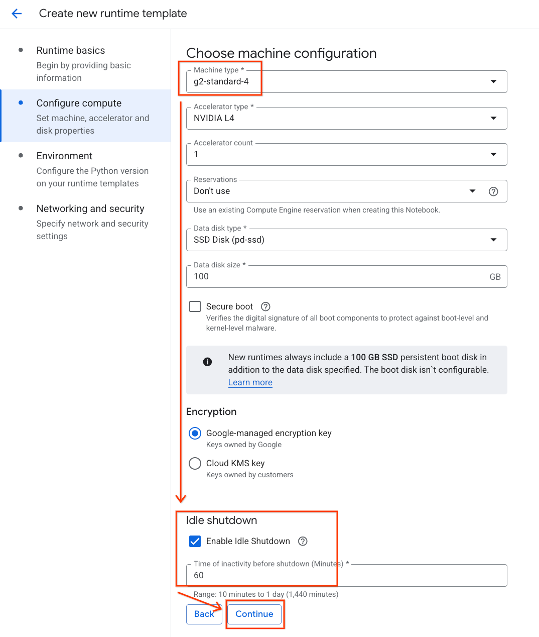
- 在「設定運算資源」下方:
- 將「Machine type」(機型) 設為
g2-standard-4。 - 將預設的「Accelerator Type」(加速器類型) 設為
NVIDIA L4,並將「Accelerator count」(加速器數量) 設為 1。 - 將「閒置關機」變更為 60 分鐘。
- 按一下「繼續」。
- 將「Machine type」(機型) 設為
- 在「環境」下方:
- 將「Environment」(環境) 設為
Python 3.11
- 將「Environment」(環境) 設為
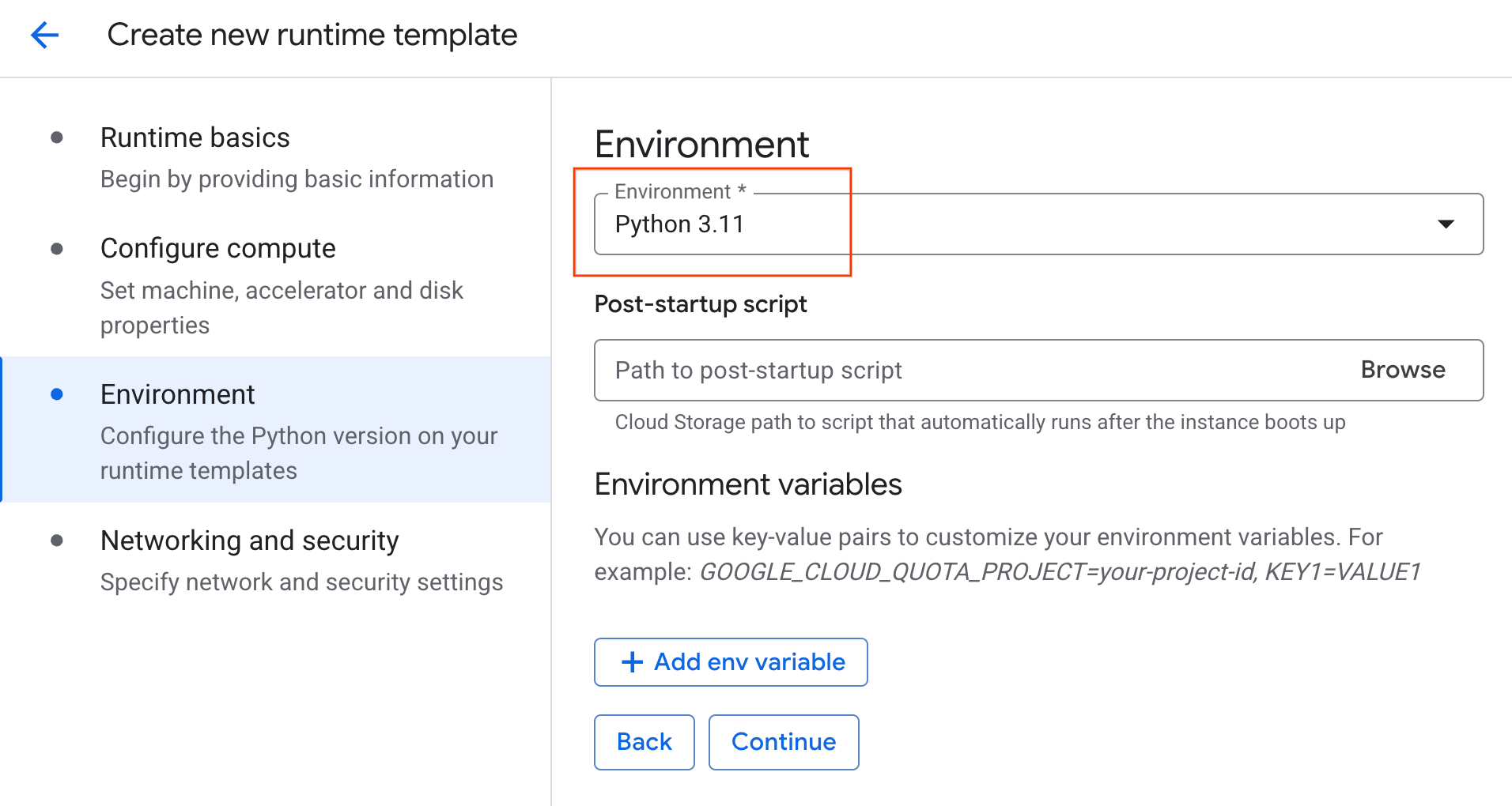
- 按一下「建立」即可儲存執行階段範本。「執行階段範本」頁面現在應該會顯示新範本。
6. 啟動執行階段
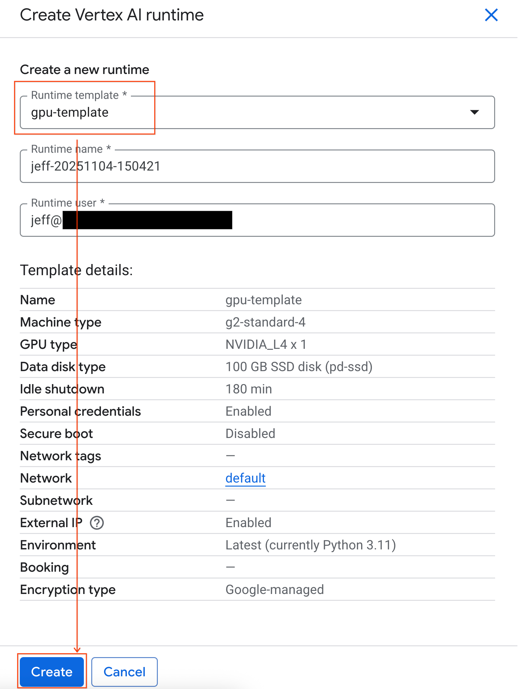
範本準備就緒後,即可建立新的執行階段。
- 在 Colab Enterprise 中,依序點選「執行階段」和「建立」。
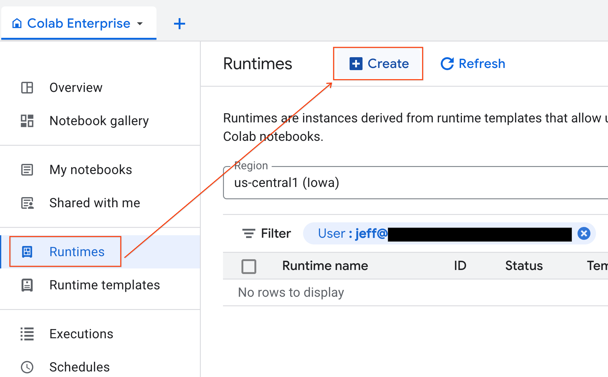
- 在「Runtime template」(執行階段範本) 下方,選取
gpu-template選項。按一下「建立」,然後等待執行階段啟動。
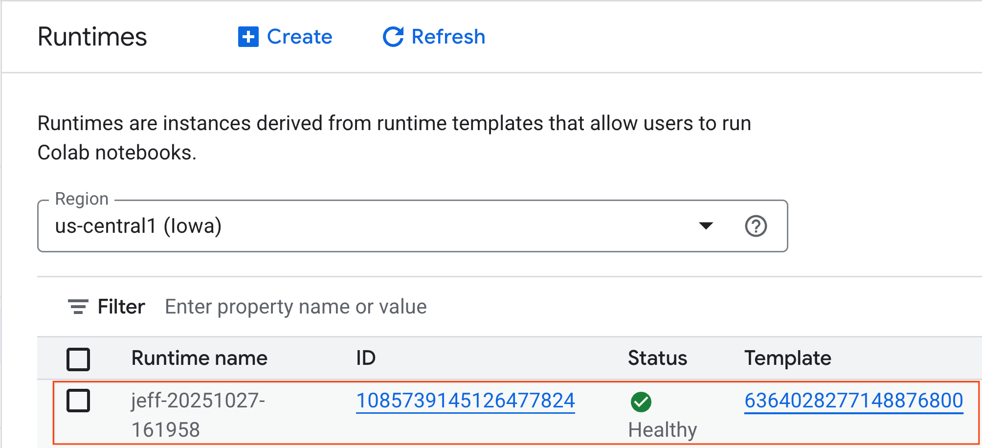
- 幾分鐘後,您就會看到可用的執行階段。
7. 設定筆記本
基礎架構執行完畢後,您需要匯入實驗室筆記本,並將其連線至執行階段。
匯入筆記本
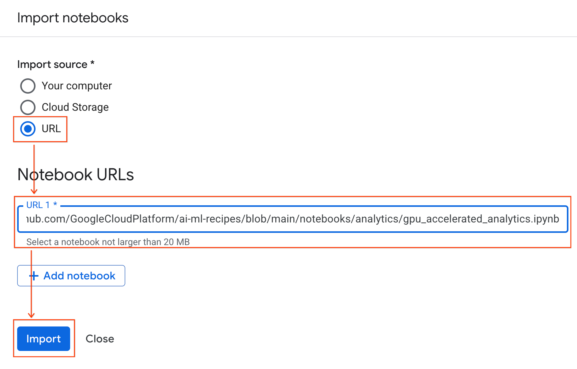
- 在 Colab Enterprise 中,依序點選「我的筆記本」和「匯入」。
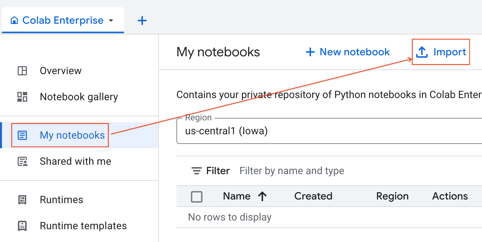
- 選取「網址」圓形按鈕,然後輸入下列網址:
https://github.com/GoogleCloudPlatform/ai-ml-recipes/blob/main/notebooks/regression/gpu_accelerated_regression/gpu_accelerated_regression.ipynb
- 按一下 [匯入]。Colab Enterprise 會將筆記本從 GitHub 複製到您的環境。
連線至執行階段
- 開啟新匯入的筆記本。
- 按一下「連結」旁的向下箭頭。
- 選取「連線到執行階段」。
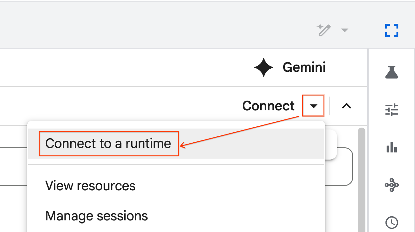
- 使用下拉式選單,選取先前建立的執行階段。
- 點選「連線」。
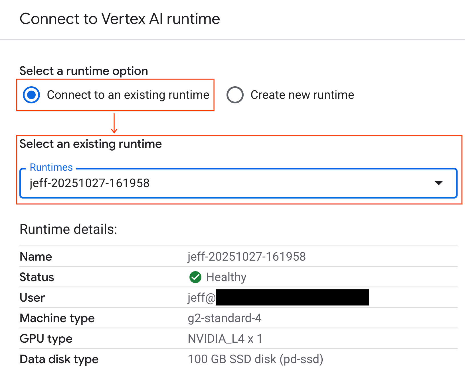
筆記本現已連線至啟用 GPU 的執行階段。
內建依附元件
使用 Colab Enterprise 的優點之一,就是系統已預先安裝您需要的程式庫。您不需要手動安裝或管理本實驗室的依附元件,例如 cuDF、cuML 或 XGBoost。
8. 準備紐約市計程車資料集
本程式碼研究室使用紐約市計程車暨禮車管理局 (TLC) 的載客記錄資料。這個資料集包含紐約市黃色計程車的行程記錄,包括:
- 取車和還車日期、時間和地點
- 行程距離
- 車資金額明細
- 乘客人數
- 小費金額 (這是我們要預測的內容!)
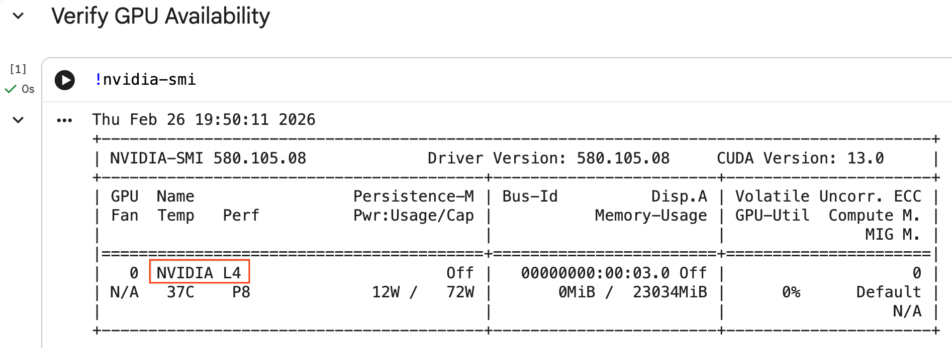
設定 GPU 並確認可用性
執行 nvidia-smi 指令,即可確認系統是否已辨識出 GPU。畫面會顯示驅動程式版本和 GPU 詳細資料 (例如 NVIDIA L4)。
nvidia-smi
儲存格應會傳回附加至執行階段的 GPU,類似如下:
下載資料
下載 2024 年的行程資料。
from tqdm import tqdm
import requests
import time
import os

YEAR = 2024
DATA_DIR = "nyc_taxi_data"

os.makedirs(DATA_DIR, exist_ok=True)
print(f"Checking/Downloading files for {YEAR}...")

for month in tqdm(range(1, 13), unit="file"):
    file_name = f"yellow_tripdata_{YEAR}-{month:02d}.parquet"
    local_path = os.path.join(DATA_DIR, file_name)
    url = f"https://d37ci6vzurychx.cloudfront.net/trip-data/{file_name}"

    if not os.path.exists(local_path):
        try:
            with requests.get(url, stream=True) as response:
                response.raise_for_status()
                with open(local_path, 'wb') as f:
                    for chunk in response.iter_content(chunk_size=8192):
                        f.write(chunk)
            time.sleep(1)
        except requests.exceptions.HTTPError as e:
            print(f"\nSkipping {file_name}: {e}")
            if os.path.exists(local_path):
                os.remove(local_path)

print("\nDownload complete.")
使用 NVIDIA cuDF 加速 pandas
pandas 程式庫會在 CPU 上執行,處理大型資料集時速度可能會較慢。NVIDIA %load_ext cudf.pandas magic 指令會動態修補 pandas,以使用 GPU 加速,並視需要改用 CPU。
我們使用這個魔法指令,而非標準匯入,因為這樣可提供「零程式碼變更」加速功能。您不必重新編寫任何現有程式碼。類似的指令 %load_ext cuml.accel 則會對 scikit-learn models 執行完全相同的操作!這項功能適用於任何具備相容 NVIDIA GPU 的 Jupyter 環境,不限於 Colab Enterprise。
%load_ext cudf.pandas
如要確認是否已啟用,請匯入 pandas 並檢查其類型:
import pandas as pd

pd
輸出內容會確認您目前使用的是 cudf.pandas 模組。
載入及清理資料
cudf.pandas 啟用後,載入 Parquet 檔案並執行資料清理作業。這項程序會在 GPU 上自動執行。
import glob

# Load data into memory
df = pd.concat(
    [pd.read_parquet(f) for f in glob.glob("nyc_taxi_data/*-01.parquet")],
    ignore_index=True
)

# Filter for valid trips. We filter for payment_type=1 (credit card)
# because tip amounts are only reliably recorded for credit card transactions.
df = df[
    (df['fare_amount'] > 0) & (df['fare_amount'] < 500) &
    (df['trip_distance'] > 0) & (df['trip_distance'] < 100) &
    (df['tip_amount'] >= 0) & (df['tip_amount'] < 100) &
    (df['payment_type'] == 1)
].copy()

# Downcast numeric columns to save memory
float_cols = df.select_dtypes(include=['float64']).columns
df[float_cols] = df[float_cols].astype('float32')

int_cols = df.select_dtypes(include=['int64']).columns
df[int_cols] = df[int_cols].astype('int32')
特徵工程
從取貨日期時間建立衍生特徵。這個筆記本包含後續步驟使用的其他功能。
import numpy as np

# Time Features
df['hour'] = df['tpep_pickup_datetime'].dt.hour
df['dow'] = df['tpep_pickup_datetime'].dt.dayofweek
df['is_weekend'] = (df['dow'] >= 5).astype(int)
df['is_rush_hour'] = (
    ((df['hour'] >= 7) & (df['hour'] <= 9)) |
    ((df['hour'] >= 17) & (df['hour'] <= 19))
).astype(int)

...
# Other features
...
9. 使用交叉驗證訓練個別模型
為說明 GPU 如何加速機器學習,您將訓練三種不同類型的迴歸模型,預測計程車行程的 tip_amount。
使用 NVIDIA cuML 加速 scikit-learn
使用 NVIDIA cuML 在 GPU 上執行 scikit-learn 演算法,無須變更 API 呼叫。首先,載入 cuml.accel 擴充功能。
%load_ext cuml.accel
設定功能和目標
找出要讓模型學習的特徵,並分割目標資料欄 (tip_amount)。
feature_cols = [
    'trip_distance', 'fare_amount', 'passenger_count',
    'hour', 'dow', 'is_weekend', 'is_rush_hour',
    'fare_log', 'fare_decimal', 'is_round_fare',
    'route_frequency', 'pu_tip_mean', 'pu_tip_std',
    'PULocationID', 'DOLocationID'
]

X = df[feature_cols].fillna(df[feature_cols].median())
y = df['tip_amount'].copy()
設定交叉驗證分割,以穩健評估模型成效。
from sklearn.model_selection import KFold
import numpy as np
import time
from sklearn.metrics import mean_squared_error
from tqdm.notebook import tqdm

n_splits = 3
kf = KFold(n_splits=n_splits, shuffle=True, random_state=42)
1. XGBoost
XGBoost 本身就支援 GPU 加速。傳遞 tree_method='hist' 和 device='cuda',在訓練期間使用 GPU。
import xgboost as xgb

start_time = time.perf_counter()

def train_xgb_cv(X, y):
    rmses = []
    preds_all = np.zeros(len(y))
    for train_idx, val_idx in tqdm(kf.split(X), total=n_splits):
        X_train, X_val = X.iloc[train_idx], X.iloc[val_idx]
        y_train, y_val = y.iloc[train_idx], y.iloc[val_idx]

        # XGBoost handles GPU natively when tree_method='hist' and device='cuda'
        model = xgb.XGBRegressor(
            objective='reg:squarederror',
            max_depth=5,
            learning_rate=0.1,
            n_estimators=100,
            tree_method='hist',
            device='cuda',
            random_state=42
        )
        model.fit(X_train, y_train)

        preds = model.predict(X_val)
        preds_all[val_idx] = preds
        rmses.append(np.sqrt(mean_squared_error(y_val, preds)))

    return np.mean(rmses), preds_all

xgb_rmse, xgb_preds = train_xgb_cv(X, y)
print(f"\n{'XGBoost RMSE:':<20} ${xgb_rmse:.4f}")
print(f"{'Time:':<20} {time.perf_counter() - start_time:.2f} seconds")
2. 線性迴歸
訓練線性迴歸模型。啟用 %load_ext cuml.accel 後,系統會自動將 LinearRegression 對應至同等效能的 GPU。
from sklearn.linear_model import LinearRegression
from sklearn.preprocessing import StandardScaler

start_time = time.perf_counter()

def train_linreg_cv(X, y):
    rmses = []
    preds_all = np.zeros(len(y))
    for train_idx, val_idx in tqdm(kf.split(X), total=n_splits):
        X_train, X_val = X.iloc[train_idx], X.iloc[val_idx]
        y_train, y_val = y.iloc[train_idx], y.iloc[val_idx]

        # Scale features
        scaler = StandardScaler()
        X_train_scaled = scaler.fit_transform(X_train)
        X_val_scaled = scaler.transform(X_val)

        # Automatically accelerated by cuML
        model = LinearRegression()
        model.fit(X_train_scaled, y_train)

        preds = model.predict(X_val_scaled)
        preds_all[val_idx] = preds
        rmses.append(np.sqrt(mean_squared_error(y_val, preds)))

    return np.mean(rmses), preds_all

linreg_rmse, linreg_preds = train_linreg_cv(X, y)
print(f"\n{'Linear Reg RMSE:':<20} ${linreg_rmse:.4f}")
print(f"{'Time:':<20} {time.perf_counter() - start_time:.2f} seconds")
3. 隨機森林
使用 RandomForestRegressor 訓練集合模型。以 CPU 訓練樹狀結構模型通常很慢,但 GPU 加速程序可更快處理數百萬列資料。
from sklearn.ensemble import RandomForestRegressor

start_time = time.perf_counter()

def train_rf_cv(X, y):
    rmses = []
    preds_all = np.zeros(len(y))
    for train_idx, val_idx in tqdm(kf.split(X), total=n_splits):
        X_train, X_val = X.iloc[train_idx], X.iloc[val_idx]
        y_train, y_val = y.iloc[train_idx], y.iloc[val_idx]

        # Automatically accelerated by cuML
        model = RandomForestRegressor(
            n_estimators=100,
            max_depth=10,
            n_jobs=-1,
            max_features='sqrt',
            random_state=42
        )
        model.fit(X_train, y_train)

        preds = model.predict(X_val)
        preds_all[val_idx] = preds
        rmses.append(np.sqrt(mean_squared_error(y_val, preds)))

    return np.mean(rmses), preds_all

rf_rmse, rf_preds = train_rf_cv(X, y)
print(f"\n{'Random Forest RMSE:':<20} ${rf_rmse:.4f}")
print(f"{'Time:':<20} {time.perf_counter() - start_time:.2f} seconds")
10. 評估端對端管道
使用簡單的線性組合,合併這三個模型的預測結果。相較於個別模型,這通常能稍微提升準確度。
對預測結果進行線性迴歸,找出最佳權重:
ensemble_weights = LinearRegression(positive=True, fit_intercept=False).fit(
    np.c_[xgb_preds, rf_preds, linreg_preds], y
).coef_

# Normalize weights
ensemble_weights = ensemble_weights / ensemble_weights.sum()

ensemble_preds = np.c_[xgb_preds, rf_preds, linreg_preds] @ ensemble_weights
ensemble_rmse = np.sqrt(mean_squared_error(y, ensemble_preds))
比較結果,即可查看集合升幅:
print(f"\n{'Model':<20} {'RMSE':>10}")
print("-" * 32)
print(f"{'Linear Regression':<20} ${linreg_rmse:>9.4f}")
print(f"{'Random Forest':<20} ${rf_rmse:>9.4f}")
print(f"{'XGBoost':<20} ${xgb_rmse:>9.4f}")
print("-" * 32)
print(f"{'Ensemble':<20} ${ensemble_rmse:>9.4f}")
print(f"\nEnsemble lift: ${xgb_rmse - ensemble_rmse:.4f}")
11. 比較 CPU 與 GPU 效能
如要正確評估效能差異,請重新啟動核心,確保執行狀態乾淨無虞,然後在 CPU 上執行整個資料科學管道,接著在 GPU 上再次執行。
重新啟動核心
執行 IPython.Application.instance().kernel.do_shutdown(True) 指令,重新啟動核心並釋放記憶體。
import IPython
IPython.Application.instance().kernel.do_shutdown(True)
定義資料科學管道
將核心工作流程 (載入資料、清理、特徵工程和模型訓練) 包裝成單一函式。這個函式會接受 pandas 模組 pd_module 和 use_gpu 引數,以便在環境之間切換。
def run_ml_pipeline(pd_module, use_gpu=False):
    import time
    import glob
    import numpy as np
    from sklearn.ensemble import RandomForestRegressor
    import xgboost as xgb

    timings = {}

    # 1. Load Data
    t0 = time.perf_counter()
    df = pd_module.concat(
        [pd_module.read_parquet(f) for f in glob.glob("nyc_taxi_data/*-01.parquet")],
        ignore_index=True
    )
    timings['Load Data'] = time.perf_counter() - t0

    # 2. Clean Data
    t0 = time.perf_counter()
    # Filter for payment_type=1 (credit card) because tip amounts
    # are only reliably recorded for credit card transactions.
    df = df[
        (df['fare_amount'] > 0) & (df['fare_amount'] < 500) &
        (df['trip_distance'] > 0) & (df['trip_distance'] < 100) &
        (df['tip_amount'] >= 0) & (df['tip_amount'] < 100) &
        (df['payment_type'] == 1)
    ].copy()

    # Downcast numeric columns to save memory
    float_cols = df.select_dtypes(include=['float64']).columns
    df[float_cols] = df[float_cols].astype('float32')
    int_cols = df.select_dtypes(include=['int64']).columns
    df[int_cols] = df[int_cols].astype('int32')
    timings['Clean Data'] = time.perf_counter() - t0

    # 3. Feature Engineering
    t0 = time.perf_counter()
    df['hour'] = df['tpep_pickup_datetime'].dt.hour
    df['dow'] = df['tpep_pickup_datetime'].dt.dayofweek
    df['is_weekend'] = (df['dow'] >= 5).astype(int)
    df['fare_log'] = np.log1p(df['fare_amount'])
    timings['Feature Engineering'] = time.perf_counter() - t0

    # 4. Modeling Prep
    feature_cols = ['trip_distance', 'fare_amount', 'passenger_count', 'hour', 'dow', 'is_weekend', 'fare_log']
    X = df[feature_cols].fillna(df[feature_cols].median())
    y = df['tip_amount'].copy()

    # Free memory
    del df
    import gc
    gc.collect()

    # 5. Train Random Forest
    t0 = time.perf_counter()
    rf_model = RandomForestRegressor(
        n_estimators=100,
        max_depth=10,
        n_jobs=-1,
        max_features='sqrt',
        random_state=42
    ).fit(X, y)
    timings['Train Random Forest'] = time.perf_counter() - t0

    # 6. Train XGBoost
    t0 = time.perf_counter()
    params = {
        'objective': 'reg:squarederror',
        'max_depth': 5,
        'n_estimators': 100,
        'random_state': 42
    }
    if use_gpu:
        params['device'] = 'cuda'
        params['tree_method'] = 'hist'
    xgb_model = xgb.XGBRegressor(**params).fit(X, y)
    timings['Train XGBoost'] = time.perf_counter() - t0

    del X
    del y
    gc.collect()

    return timings
在 CPU 上執行
使用標準 CPU pandas 呼叫管道。
import pandas as pd

print("Running pipeline on CPU...")
cpu_times = run_ml_pipeline(pd, use_gpu=False)
print("CPU Execution Finished.")
在 GPU 上執行
載入 NVIDIA 程式庫擴充功能、將加速的 cudf.pandas 模組傳遞至管道,並在內部將 XGBoost 裝置設為 cuda。
import IPython.core.magic
if not hasattr(IPython.core.magic, 'output_can_be_silenced'):
    IPython.core.magic.output_can_be_silenced = lambda x: x

%load_ext cudf.pandas
%load_ext cuml.accel
import pandas as pd

print("Running pipeline on GPU...")
gpu_times = run_ml_pipeline(pd, use_gpu=True)
print("GPU Execution Finished.")
以圖表呈現效能加速
使用 matplotlib 顯示時間。結果會顯示使用 GPU 時,在資料處理和模型訓練期間節省的時間。
import matplotlib.pyplot as plt
import numpy as np

labels = list(cpu_times.keys())
cpu_values = list(cpu_times.values())
gpu_values = list(gpu_times.values())

x = np.arange(len(labels))
width = 0.35

fig, ax = plt.subplots(figsize=(10, 6))
rects1 = ax.bar(x - width/2, cpu_values, width, label='CPU', color='#4285F4')
rects2 = ax.bar(x + width/2, gpu_values, width, label='GPU', color='#76B900')

ax.set_ylabel('Execution Time (seconds)')
ax.set_title('NYC Taxi ML Pipeline: CPU vs. GPU Performance')
ax.set_xticks(x)
ax.set_xticklabels(labels, rotation=45, ha="right")
ax.legend()

# Add data labels
def autolabel(rects):
    for rect in rects:
        height = rect.get_height()
        ax.annotate(f'{height:.2f}s',
                    xy=(rect.get_x() + rect.get_width() / 2, height),
                    xytext=(0, 3),  # 3 points vertical offset
                    textcoords="offset points",
                    ha='center', va='bottom', fontsize=9)
autolabel(rects1)
autolabel(rects2)

plt.tight_layout()
plt.show()

# Calculate overall speedup
total_cpu_time = sum(cpu_values)
total_gpu_time = sum(gpu_values)
overall_speedup = total_cpu_time / total_gpu_time
print(f"\nOverall Pipeline Speedup: {overall_speedup:.2f}x faster on GPU!")
您應該會看到類似下方的內容:
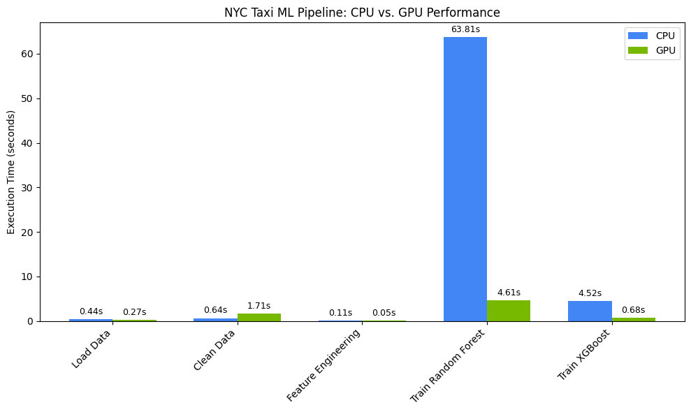
這張圖表說明 GPU 在整個資料科學工作流程中,效能顯著優於 CPU。對於隨機森林和 XGBoost 等演算法,您應該會在運算密集型模型訓練階段,看到最顯著的節省時間效果。
12. 分析程式碼,找出效能限制
使用 cudf.pandas 時,大多數函式都會在 GPU 上執行。如果 cuDF 尚未支援特定作業,執行作業會暫時改回使用 CPU。NVIDIA 提供兩個內建的 Jupyter 神奇指令,可識別這些備援。
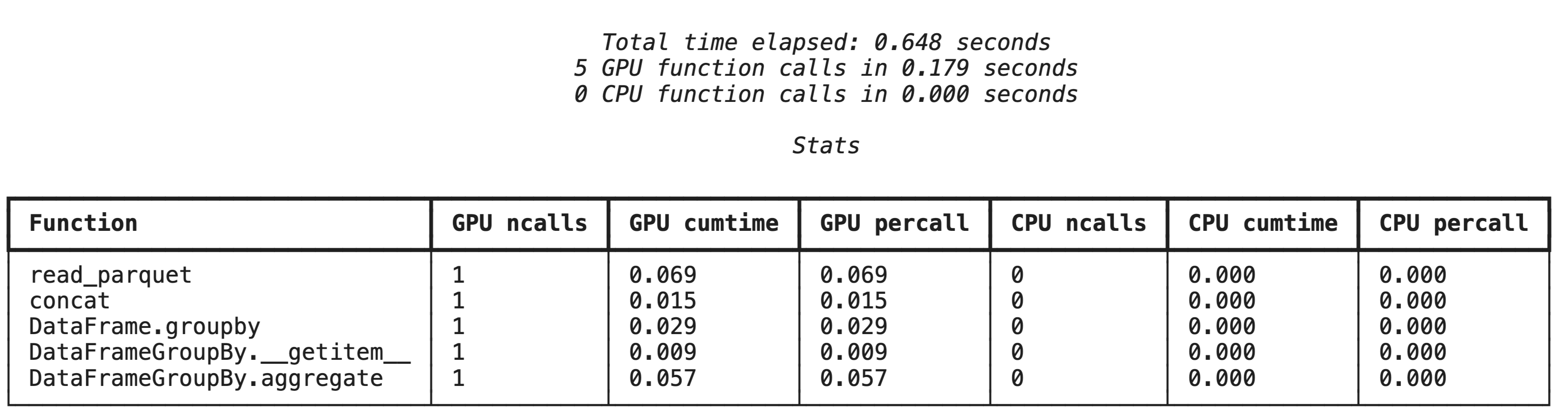
使用 %%cudf.pandas.profile 進行高層級剖析
%%cudf.pandas.profile 魔法指令會提供摘要,說明哪些函式在 GPU 或 CPU 上執行。
%%cudf.pandas.profile

import glob
import pandas as pd

df = pd.concat([pd.read_parquet(f) for f in glob.glob("nyc_taxi_data/*-01.parquet")], ignore_index=True)

summary = (
    df
      .groupby(['PULocationID', 'payment_type'])
      [['passenger_count', 'fare_amount', 'tip_amount']]
      .agg(['min', 'mean', 'max'])
)
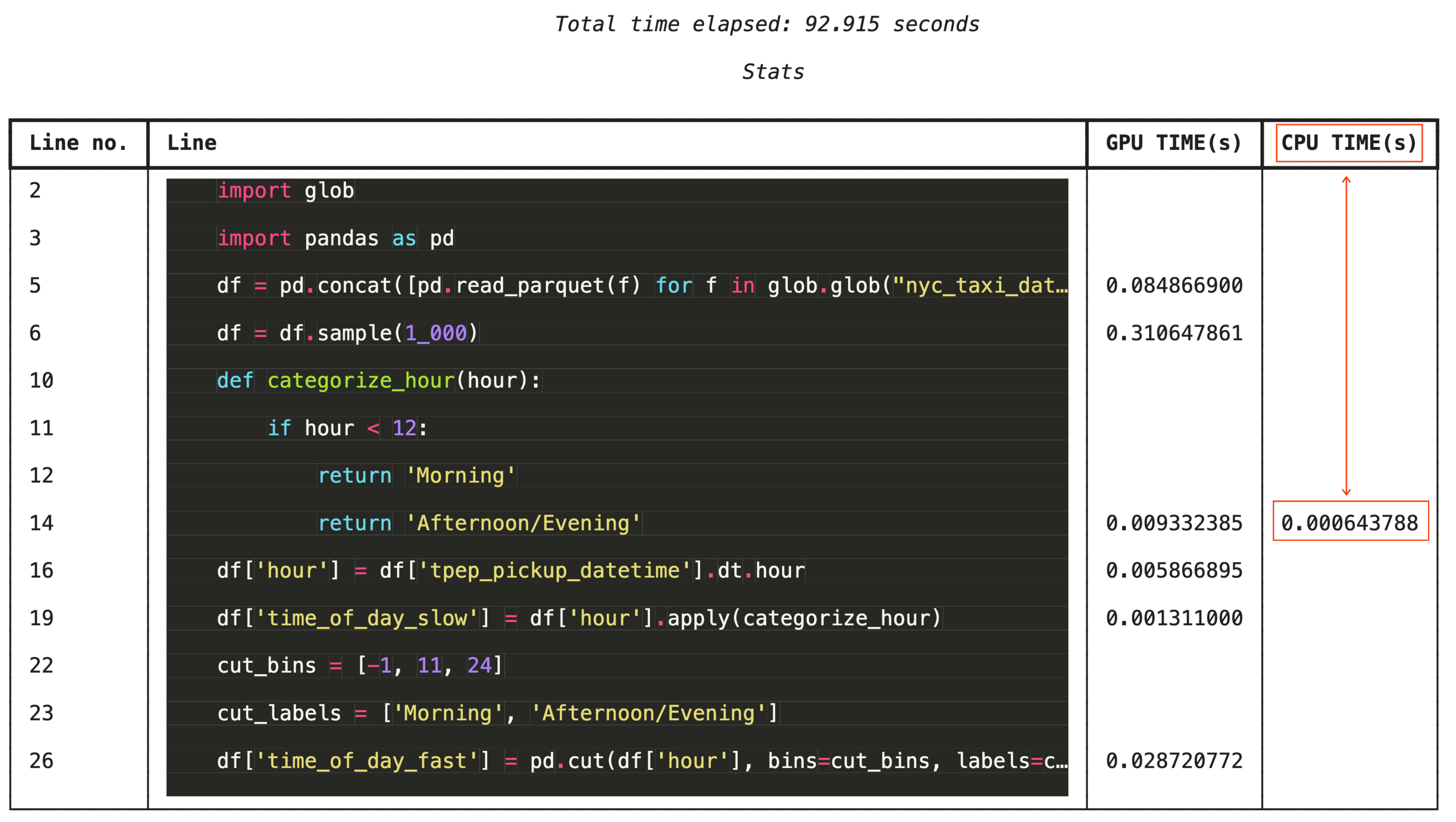
使用 %%cudf.pandas.line_profile 逐行分析
如要進行精細疑難排解,%%cudf.pandas.line_profile 會在每行程式碼中標註,標示該行程式碼在 GPU 和 CPU 上執行的次數。
%%cudf.pandas.line_profile

import glob
import pandas as pd

df = pd.concat([pd.read_parquet(f) for f in glob.glob("nyc_taxi_data/*-01.parquet")], ignore_index=True)
df = df.sample(1_000)

# Iterating row-by-row or using custom python apply functions often falls back to the CPU
def categorize_hour(hour):
    if hour < 12:
        return 'Morning'
    else:
        return 'Afternoon/Evening'

df['hour'] = df['tpep_pickup_datetime'].dt.hour

df['time_of_day_slow'] = df['hour'].apply(categorize_hour)

# Using vectorized pandas operations (like pd.cut) stays entirely on the GPU
cut_bins = [-1, 11, 24]
cut_labels = ['Morning', 'Afternoon/Evening']
df['time_of_day_fast'] = pd.cut(df['hour'], bins=cut_bins, labels=cut_labels)
13. 清除
為避免 Google Cloud 帳戶產生預期外的費用,請清理在本程式碼實驗室建立的資源。
刪除資源
在筆記本儲存格中,使用 !rm -rf 指令刪除執行階段的本機資料集。
print("Deleting local 'nyc_taxi_data' directory...")
!rm -rf nyc_taxi_data
print("Local files deleted.")
關閉 Colab 執行階段
- 前往 Google Cloud 控制台的 Colab Enterprise「執行階段」頁面。
- 在「Region」(區域) 選單中,選取包含執行階段的區域。
- 選取要刪除的執行階段。
- 按一下「刪除」。
- 按一下「確認」。
刪除筆記本
- 前往 Google Cloud 控制台的 Colab Enterprise「我的筆記本」頁面。
- 在「Region」(區域) 選單中,選取包含筆記本的區域。
- 選取要刪除的記事本。
- 按一下「刪除」。
- 按一下「確認」。
14. 恭喜
恭喜!您已成功在 Colab Enterprise 上使用 NVIDIA cuDF 和 cuML 程式庫,加速 pandas 和 scikit-learn 機器學習工作流程。只要新增幾個魔法指令 (%load_ext cudf.pandas 和 %load_ext cuml.accel),標準程式碼就能在 GPU 上執行,以極短的時間處理記錄並在本地擬合複雜模型。
如要進一步瞭解如何使用 GPU 加速資料分析,請參閱「Accelerated Data Analytics with GPUs」程式碼研究室。
涵蓋內容
- 瞭解 Google Cloud 上的 Colab Enterprise。
- 使用特定 GPU 和記憶體設定自訂 Colab 執行階段環境。
- 使用紐約市計程車資料集中的數百萬筆記錄,套用 GPU 加速功能來預測小費金額。
- 使用 NVIDIA 的
cuDF程式庫,在完全不修改程式碼的情況下加速pandas。 - 使用 NVIDIA 的
cuML程式庫和 GPU,在不變更任何程式碼的情況下加速scikit-learn。 - 剖析程式碼,找出並最佳化效能限制。