
1. 개요
이 실습에서는 BigQuery Studio의 Python 노트북에서 BigQuery DataFrames를 사용하여 아이오와 주류 판매 공개 데이터 세트를 정리하고 분석합니다. BigQuery ML 및 원격 함수 기능을 활용하여 유용한 정보를 발견합니다.
Python 노트북을 만들어 지리적 영역 간 판매를 비교합니다. 이는 모든 구조화된 데이터에서 작동하도록 조정할 수 있습니다.
목표
이 실습에서는 다음 작업을 수행하는 방법을 알아봅니다.
- BigQuery Studio에서 Python 노트북 활성화 및 사용
- BigQuery DataFrame 패키지를 사용하여 BigQuery에 연결
- BigQuery ML을 사용하여 선형 회귀 만들기
- 친숙한 pandas와 유사한 문법을 사용하여 복잡한 집계 및 조인 실행
2. 요구사항
시작하기 전에
이 Codelab의 안내를 따르려면 BigQuery Studio가 사용 설정되어 있고 연결된 결제 계정이 있는 Google Cloud 프로젝트가 필요합니다.
- Google Cloud 콘솔의 프로젝트 선택기 페이지에서 Google Cloud 프로젝트를 선택하거나 만듭니다.
- Google Cloud 프로젝트에 결제가 사용 설정되어 있는지 확인합니다. 프로젝트에 결제가 사용 설정되어 있는지 확인하는 방법을 알아보세요.
- 안내에 따라 애셋 관리에 BigQuery Studio를 사용 설정합니다.
BigQuery Studio 준비
빈 노트북을 만들고 런타임에 연결합니다.
- Google Cloud 콘솔에서 BigQuery Studio로 이동합니다.
- + 버튼 옆에 있는 ▼를 클릭합니다.
- Python 노트북을 선택합니다.
- 템플릿 선택기를 닫습니다.
- + 코드를 선택하여 새 코드 셀을 만듭니다.
- 코드 셀에서 최신 버전의 BigQuery DataFrames 패키지를 설치합니다.다음 명령어를 입력합니다.
%pip install --upgrade bigframes --quiet
3. 공개 데이터 세트 읽기
새 코드 셀에서 다음을 실행하여 BigQuery DataFrames 패키지를 초기화합니다.
import bigframes.pandas as bpd

bpd.options.bigquery.ordering_mode = "partial"
bpd.options.display.repr_mode = "deferred"
참고: 이 튜토리얼에서는 실험적인 '부분 순서 지정 모드'를 사용합니다. 이 모드는 pandas와 유사한 필터링과 함께 사용할 때 더 효율적인 쿼리를 허용합니다. 엄격한 순서 지정이나 색인이 필요한 일부 pandas 기능은 작동하지 않을 수 있습니다.
다음 명령어를 사용하여 bigframes 패키지 버전을 확인합니다.
bpd.__version__
이 가이드에는 버전 1.27.0 이상이 필요합니다.
아이오와 주류 소매 판매
아이오와주 주류 소매 판매 데이터 세트는 Google Cloud의 공개 데이터 세트 프로그램을 통해 BigQuery에서 제공됩니다. 이 데이터 세트에는 2012년 1월 1일 이후 아이오와주에서 소매업체가 개인에게 판매하기 위해 구매한 모든 주류 도매 구매가 포함되어 있습니다. 데이터는 아이오와주 상무부 내 주류 부서에서 수집합니다.
BigQuery에서 bigquery-public-data.iowa_liquor_sales.sales를 쿼리하여 아이오와 주류 소매 판매를 분석합니다. bigframes.pandas.read_gbq() 메서드를 사용하여 쿼리 문자열 또는 테이블 ID에서 DataFrame을 만듭니다.
새 코드 셀에서 다음을 실행하여 'df'라는 DataFrame을 만듭니다.
df = bpd.read_gbq_table("bigquery-public-data.iowa_liquor_sales.sales")
DataFrame에 관한 기본 정보 알아보기
DataFrame.peek() 메서드를 사용하여 소규모 데이터 샘플을 다운로드합니다.
이 셀을 실행합니다.
df.peek()
예상 출력:
index	invoice_and_item_number	date	store_number	store_name	...
0	RINV-04620300080	2023-04-28	10197	SUNSHINE FOODS / HAWARDEN
1	RINV-04864800097	2023-09-25	2621	HY-VEE FOOD STORE #3 / SIOUX CITY
2	RINV-05057200028	2023-12-28	4255	FAREWAY STORES #058 / ORANGE CITY
3	...
참고: head()에는 순서가 필요하며 데이터 샘플을 시각화하려는 경우 일반적으로 peek()보다 효율성이 떨어집니다.
pandas와 마찬가지로 DataFrame.dtypes 속성을 사용하여 사용 가능한 모든 열과 해당 데이터 유형을 확인할 수 있습니다. 이러한 값은 pandas와 호환되는 방식으로 노출됩니다.
이 셀을 실행합니다.
df.dtypes
예상 출력:
invoice_and_item_number	string[pyarrow]
date	date32[day][pyarrow]
store_number	string[pyarrow]
store_name	string[pyarrow]
address	string[pyarrow]
city	string[pyarrow]
zip_code	string[pyarrow]
store_location	geometry
county_number	string[pyarrow]
county	string[pyarrow]
category	string[pyarrow]
category_name	string[pyarrow]
vendor_number	string[pyarrow]
vendor_name	string[pyarrow]
item_number	string[pyarrow]
item_description	string[pyarrow]
pack	Int64
bottle_volume_ml	Int64
state_bottle_cost	Float64
state_bottle_retail	Float64
bottles_sold	Int64
sale_dollars	Float64
volume_sold_liters	Float64
volume_sold_gallons	Float64

dtype: object
DataFrame.describe() 메서드는 DataFrame에서 몇 가지 기본 통계를 쿼리합니다. DataFrame.to_pandas()을 실행하여 이러한 요약 통계를 pandas DataFrame으로 다운로드합니다.
이 셀을 실행합니다.
df.describe("all").to_pandas()
예상 출력:
	invoice_and_item_number	date	store_number	store_name	...
nunique	30305765	<NA>	3158	3353	...
std	<NA>	<NA>	<NA>	<NA>	...
mean	<NA>	<NA>	<NA>	<NA>	...
75%	<NA>	<NA>	<NA>	<NA>	...
25%	<NA>	<NA>	<NA>	<NA>	...
count	30305765	<NA>	30305765	30305765	...
min	<NA>	<NA>	<NA>	<NA>	...
50%	<NA>	<NA>	<NA>	<NA>	...
max	<NA>	<NA>	<NA>	<NA>	...
9 rows × 24 columns
4. 데이터 시각화 및 정리
아이오와 주류 소매 판매 데이터 세트는 소매점이 있는 위치를 비롯한 세부적인 지리 정보를 제공합니다. 이 데이터를 사용하여 지역 간 추세와 차이를 파악합니다.
우편번호별 판매 시각화
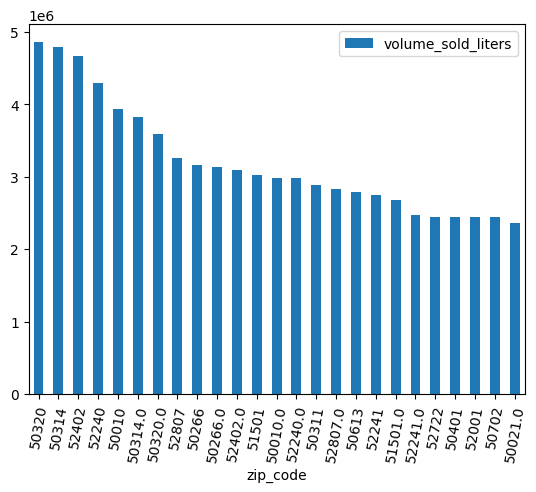
DataFrame.plot.hist()와 같은 여러 기본 시각화 메서드가 있습니다. 이 메서드를 사용하여 우편번호별 주류 판매를 비교하세요.
volume_by_zip = df.groupby("zip_code").agg({"volume_sold_liters": "sum"})
volume_by_zip.plot.hist(bins=20)
예상 출력:

막대 그래프를 사용하여 어떤 우편번호에서 알코올이 가장 많이 판매되었는지 확인합니다.
(
  volume_by_zip
  .sort_values("volume_sold_liters", ascending=False)
  .head(25)
  .to_pandas()
  .plot.bar(rot=80)
)
예상 출력:
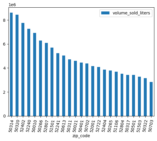
데이터 정리
일부 우편번호에는 .0가 있습니다. 데이터 수집 과정에서 우편번호가 실수로 부동 소수점 값으로 변환되었을 수 있습니다. 정규 표현식을 사용하여 우편번호를 정리하고 분석을 반복합니다.
df = (
    bpd.read_gbq_table("bigquery-public-data.iowa_liquor_sales.sales")
    .assign(
        zip_code=lambda _: _["zip_code"].str.replace(".0", "")
    )
)
volume_by_zip = df.groupby("zip_code").agg({"volume_sold_liters": "sum"})
(
  volume_by_zip
  .sort_values("volume_sold_liters", ascending=False)
  .head(25)
  .to_pandas()
  .plot.bar(rot=80)
)
예상 출력:
5. 매출의 상관관계 파악
일부 우편번호에서 다른 우편번호보다 더 많이 판매되는 이유는 무엇인가요? 한 가지 가설은 인구수 차이 때문이라는 것입니다. 인구가 많은 우편번호에서는 주류가 더 많이 판매될 가능성이 높습니다.
인구와 주류 판매량 간의 상관관계를 계산하여 이 가설을 테스트합니다.
다른 데이터 세트와 조인
미국 인구조사국의 미국 지역사회 설문조사 우편번호 표 형식 영역 설문조사와 같은 인구 데이터 세트와 조인합니다.
census_acs = bpd.read_gbq_table("bigquery-public-data.census_bureau_acs.zcta_2020_5yr")
American Community Survey는 GEOID로 주를 식별합니다. 우편번호 표 영역의 경우 GEOID는 우편번호와 같습니다.
volume_by_pop = volume_by_zip.join(
    census_acs.set_index("geo_id")
)
우편번호 집계 지역 인구와 판매된 알코올 리터를 비교하는 산점도를 만듭니다.
(
    volume_by_pop[["volume_sold_liters", "total_pop"]]
    .to_pandas()
    .plot.scatter(x="total_pop", y="volume_sold_liters")
)
예상 출력:
상관관계 계산
추세는 대략 선형으로 보입니다. 여기에 선형 회귀 모델을 적합시켜 인구가 주류 판매량을 얼마나 잘 예측할 수 있는지 확인합니다.
from bigframes.ml.linear_model import LinearRegression

feature_columns = volume_by_pop[["total_pop"]]
label_columns = volume_by_pop[["volume_sold_liters"]]

# Create the linear model
model = LinearRegression()
model.fit(feature_columns, label_columns)
score 메서드를 사용하여 적합성을 확인합니다.
model.score(feature_columns, label_columns).to_pandas()
샘플 출력:
	mean_absolute_error	mean_squared_error	mean_squared_log_error	median_absolute_error	r2_score	explained_variance
0	245065.664095	224398167097.364288	5.595021	178196.31289	0.380096	0.380096
모집단 값 범위에서 predict 함수를 호출하여 최적선 그리기
import matplotlib.pyplot as pyplot
import numpy as np
import pandas as pd

line = pd.Series(np.arange(0, 50_000), name="total_pop")
predictions = model.predict(line).to_pandas()

zips = volume_by_pop[["volume_sold_liters", "total_pop"]].to_pandas()
pyplot.scatter(zips["total_pop"], zips["volume_sold_liters"])
pyplot.plot(
  line,
  predictions.sort_values("total_pop")["predicted_volume_sold_liters"],
  marker=None,
  color="red",
)
예상 출력:
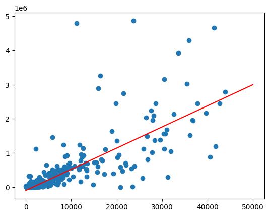
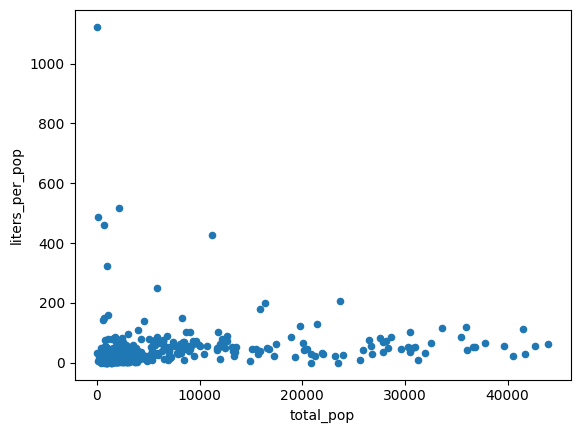
이분산성 해결
이전 차트의 데이터는 이분산성인 것으로 보입니다. 최적선 주변의 분산은 인구와 함께 증가합니다.
1인당 구매하는 알코올의 양은 비교적 일정할 수 있습니다.
volume_per_pop = (
    volume_by_pop[volume_by_pop['total_pop'] > 0]
    .assign(liters_per_pop=lambda df: df["volume_sold_liters"] / df["total_pop"])
)

(
    volume_per_pop[["liters_per_pop", "total_pop"]]
    .to_pandas()
    .plot.scatter(x="total_pop", y="liters_per_pop")
)
예상 출력:
다음 두 가지 방법으로 구매한 평균 알코올 리터를 계산합니다.
- 아이오와에서 1인당 구매하는 알코올의 평균량은 얼마인가요?
- 모든 우편번호에서 1인당 구매한 알코올의 평균량은 얼마인가요?
(1)에서는 주 전체에서 구매한 알코올의 양을 반영합니다. (2)에서는 평균 우편번호를 반영하며, 우편번호마다 인구가 다르기 때문에 (1)과 반드시 동일하지는 않습니다.
df = (
    bpd.read_gbq_table("bigquery-public-data.iowa_liquor_sales.sales")
    .assign(
        zip_code=lambda _: _["zip_code"].str.replace(".0", "")
    )
)
census_state = bpd.read_gbq(
    "bigquery-public-data.census_bureau_acs.state_2020_5yr",
    index_col="geo_id",
)

volume_per_pop_statewide = (
    df['volume_sold_liters'].sum()
    / census_state["total_pop"].loc['19']
)
volume_per_pop_statewide
예상 출력: 87.997
average_per_zip = volume_per_pop["liters_per_pop"].mean()
average_per_zip
예상 출력: 67.139
위와 마찬가지로 이러한 평균을 표시합니다.
import numpy as np
import pandas as pd
from matplotlib import pyplot

line = pd.Series(np.arange(0, 50_000), name="total_pop")

zips = volume_per_pop[["liters_per_pop", "total_pop"]].to_pandas()
pyplot.scatter(zips["total_pop"], zips["liters_per_pop"])
pyplot.plot(line, np.full(line.shape, volume_per_pop_statewide), marker=None, color="magenta")
pyplot.plot(line, np.full(line.shape, average_per_zip), marker=None, color="red")
예상 출력:
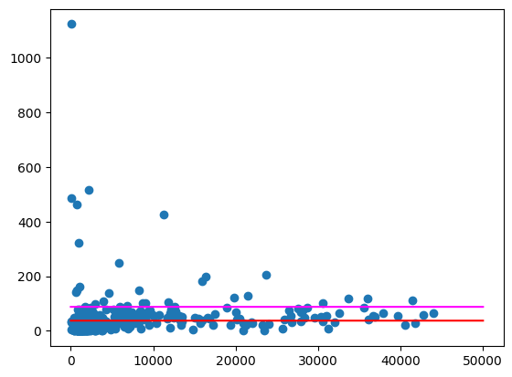
특히 인구가 적은 지역에는 여전히 상당히 큰 이상치가 있는 우편번호가 있습니다. 이러한 현상이 발생하는 이유를 추측하는 것은 연습 문제로 남겨 두겠습니다. 예를 들어 일부 우편번호에는 인구가 적지만 해당 지역에 유일한 주류 판매점이 있어 소비량이 많을 수 있습니다. 이 경우 주변 우편번호의 인구를 기반으로 계산하면 이러한 이상치를 균등하게 처리할 수 있습니다.
6. 판매된 주류 유형 비교
아이오와 주류 소매 판매 데이터베이스에는 지리적 데이터 외에도 판매된 상품에 대한 세부정보가 포함되어 있습니다. 이러한 데이터를 분석하면 지역별 취향의 차이를 파악할 수 있습니다.
카테고리 탐색하기
데이터베이스에서 항목이 분류됩니다. 카테고리가 몇 개 있나요?
import bigframes.pandas as bpd

bpd.options.bigquery.ordering_mode = "partial"
bpd.options.display.repr_mode = "deferred"

df = bpd.read_gbq_table("bigquery-public-data.iowa_liquor_sales.sales")
df.category_name.nunique()
예상 출력: 103
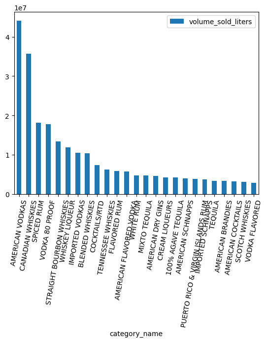
가장 인기 있는 카테고리는 무엇인가요?
counts = (
    df.groupby("category_name")
    .agg({"volume_sold_liters": "sum"})
    .sort_values(["volume_sold_liters"], ascending=False)
    .to_pandas()
)
counts.head(25).plot.bar(rot=80)
ARRAY 데이터 유형 작업
위스키, 럼, 보드카 등 다양한 카테고리가 있습니다. 이러한 항목을 어떻게든 그룹화하고 싶습니다.
Series.str.split() 메서드를 사용하여 카테고리 이름을 별도의 단어로 분할하는 것으로 시작합니다. explode() 메서드를 사용하여 이 메서드로 생성된 배열을 중첩 해제합니다.
category_parts = df.category_name.str.split(" ").explode()
counts = (
    category_parts
    .groupby(category_parts)
    .size()
    .sort_values(ascending=False)
    .to_pandas()
)
counts.head(25).plot.bar(rot=80)
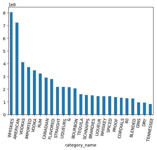
category_parts.nunique()
예상 출력: 113
위 차트를 보면 데이터에 VODKA와 VODKAS가 별도로 표시됩니다. 카테고리를 더 작은 집합으로 접으려면 더 많은 그룹화가 필요합니다.
7. BigQuery DataFrames와 함께 NLTK 사용
카테고리가 100개 정도밖에 되지 않으므로 휴리스틱을 작성하거나 카테고리에서 더 넓은 주류 유형으로의 매핑을 수동으로 만드는 것이 가능합니다. 또는 Gemini와 같은 대규모 언어 모델을 사용하여 이러한 매핑을 만들 수 있습니다. BigQuery DataFrames를 사용하여 구조화되지 않은 데이터에서 인사이트 얻기 Codelab을 통해 Gemini와 함께 BigQuery DataFrames를 사용해 보세요.
대신 더 전통적인 자연어 처리 패키지인 NLTK를 사용하여 이 데이터를 처리하세요. 예를 들어 '어간 추출기'라는 기술을 사용하면 복수 명사와 단수 명사를 동일한 값으로 병합할 수 있습니다.
NLTK를 사용하여 단어 어간 추출
NLTK 패키지는 Python에서 액세스할 수 있는 자연어 처리 방법을 제공합니다. 패키지를 설치하여 사용해 보세요.
%pip install nltk
다음으로 패키지를 가져옵니다. 버전을 검사합니다. 이 값은 튜토리얼 뒷부분에서 사용됩니다.
import nltk

nltk.__version__
단어를 표준화하여 단어의 '어간'을 만드는 한 가지 방법입니다. 이렇게 하면 복수형의 끝에 오는 's'와 같은 접미사가 삭제됩니다.
def stem(word: str) -> str:
    # https://www.nltk.org/howto/stem.html
    import nltk.stem.snowball

    # Avoid failure if a NULL is passed in.
    if not word:
        return word

    stemmer = nltk.stem.snowball.SnowballStemmer("english")
    return stemmer.stem(word)
몇 단어에 적용해 보세요.
stem("WHISKEY")
예상 출력: whiskey
stem("WHISKIES")
예상 출력: whiski
안타깝게도 위스키가 위스키와 동일하게 매핑되지 않았습니다. 어간 추출기는 불규칙 복수형과 잘 작동하지 않습니다. 더 정교한 기술을 사용하여 '표제어'라고 하는 기본 단어를 식별하는 표제어 추출기를 사용해 보세요.
def lemmatize(word: str) -> str:
    # https://stackoverflow.com/a/18400977/101923
    # https://www.nltk.org/api/nltk.stem.wordnet.html#module-nltk.stem.wordnet
    import nltk
    import nltk.stem.wordnet


    # Avoid failure if a NULL is passed in.
    if not word:
        return word

    nltk.download('wordnet')
    wnl = nltk.stem.wordnet.WordNetLemmatizer()
    return wnl.lemmatize(word.lower())
몇 단어에 적용해 보세요.
lemmatize("WHISKIES")
예상 출력: whisky
lemmatize("WHISKY")
예상 출력: whisky
lemmatize("WHISKEY")
예상 출력: whiskey
안타깝게도 이 표제어 추출기는 'whiskey'를 'whiskies'와 동일한 표제어로 매핑하지 않습니다. 이 단어는 아이오와 소매 주류 판매 데이터베이스에서 특히 중요하므로 사전을 사용하여 미국식 철자에 수동으로 매핑합니다.
def lemmatize(word: str) -> str:
    # https://stackoverflow.com/a/18400977/101923
    # https://www.nltk.org/api/nltk.stem.wordnet.html#module-nltk.stem.wordnet
    import nltk
    import nltk.stem.wordnet


    # Avoid failure if a NULL is passed in.
    if not word:
        return word

    nltk.download('wordnet')
    wnl = nltk.stem.wordnet.WordNetLemmatizer()
    lemma = wnl.lemmatize(word.lower())

    table = {
        "whisky": "whiskey",  # Use the American spelling.
    }
    return table.get(lemma, lemma)
몇 단어에 적용해 보세요.
lemmatize("WHISKIES")
예상 출력: whiskey
lemmatize("WHISKEY")
예상 출력: whiskey
축하합니다. 이 표제어 추출기는 카테고리를 좁히는 데 적합합니다. BigQuery와 함께 사용하려면 클라우드에 배포해야 합니다.
함수 배포를 위한 프로젝트 설정
BigQuery가 이 함수에 액세스할 수 있도록 클라우드에 배포하기 전에 일회성 설정을 해야 합니다.
새 코드 셀을 만들고 your-project-id를 이 튜토리얼에서 사용하는 Google Cloud 프로젝트 ID로 바꿉니다.
project_id = "your-project-id"
이 함수는 클라우드 리소스에 액세스할 필요가 없으므로 권한이 없는 서비스 계정을 만듭니다.
from google.cloud import iam_admin_v1
from google.cloud.iam_admin_v1 import types

iam_admin_client = iam_admin_v1.IAMClient()
request = types.CreateServiceAccountRequest()

account_id = "bigframes-no-permissions"
request.account_id = account_id
request.name = f"projects/{project_id}"

display_name = "bigframes remote function (no permissions)"
service_account = types.ServiceAccount()
service_account.display_name = display_name
request.service_account = service_account

account = iam_admin_client.create_service_account(request=request)
print(account.email)
예상 출력: bigframes-no-permissions@your-project-id.iam.gserviceaccount.com
함수를 저장할 BigQuery 데이터 세트를 만듭니다.
from google.cloud import bigquery

bqclient = bigquery.Client(project=project_id)
dataset = bigquery.Dataset(f"{project_id}.functions")
bqclient.create_dataset(dataset, exists_ok=True)
원격 함수 배포
아직 사용 설정하지 않은 경우 Cloud Functions API를 사용 설정합니다.
!gcloud services enable cloudfunctions.googleapis.com
이제 방금 만든 데이터 세트에 함수를 배포합니다. 이전 단계에서 만든 함수에 @bpd.remote_function 데코레이터를 추가합니다.
@bpd.remote_function(
    dataset=f"{project_id}.functions",
    name="lemmatize",
    # TODO: Replace this with your version of nltk.
    packages=["nltk==3.9.1"],
    cloud_function_service_account=f"bigframes-no-permissions@{project_id}.iam.gserviceaccount.com",
    cloud_function_ingress_settings="internal-only",
)
def lemmatize(word: str) -> str:
    # https://stackoverflow.com/a/18400977/101923
    # https://www.nltk.org/api/nltk.stem.wordnet.html#module-nltk.stem.wordnet
    import nltk
    import nltk.stem.wordnet


    # Avoid failure if a NULL is passed in.
    if not word:
        return word

    nltk.download('wordnet')
    wnl = nltk.stem.wordnet.WordNetLemmatizer()
    lemma = wnl.lemmatize(word.lower())

    table = {
        "whisky": "whiskey",  # Use the American spelling.
    }
    return table.get(lemma, lemma)
배포하는 데 약 2분이 소요됩니다.
원격 기능 사용
배포가 완료되면 이 함수를 테스트할 수 있습니다.
lemmatize = bpd.read_gbq_function(f"{project_id}.functions.lemmatize")

words = bpd.Series(["whiskies", "whisky", "whiskey", "vodkas", "vodka"])
words.apply(lemmatize).to_pandas()
예상 출력:
0	whiskey
1	whiskey
2	whiskey
3	vodka
4	vodka

dtype: string
8. 군별 알코올 소비량 비교
이제 lemmatize 함수를 사용할 수 있으므로 이를 사용하여 카테고리를 결합합니다.
카테고리를 가장 잘 요약하는 단어 찾기
먼저 데이터베이스의 모든 카테고리로 DataFrame을 만듭니다.
df = bpd.read_gbq_table("bigquery-public-data.iowa_liquor_sales.sales")

categories = (
    df['category_name']
    .groupby(df['category_name'])
    .size()
    .to_frame()
    .rename(columns={"category_name": "total_orders"})
    .reset_index(drop=False)
)
categories.to_pandas()
예상 출력:
category_name	total_orders
0	100 PROOF VODKA	99124
1	100% AGAVE TEQUILA	724374
2	AGED DARK RUM	59433
3	AMARETTO - IMPORTED	102
4	AMERICAN ALCOHOL	24351
...	...	...
98	WATERMELON SCHNAPPS	17844
99	WHISKEY LIQUEUR	1442732
100	WHITE CREME DE CACAO	7213
101	WHITE CREME DE MENTHE	2459
102	WHITE RUM	436553
103 rows × 2 columns
다음으로 구두점, 'item'과 같은 몇 가지 필러 단어를 제외한 카테고리의 모든 단어로 DataFrame을 만듭니다.
words = (
    categories.assign(
        words=categories['category_name']
        .str.lower()
        .str.split(" ")
    )
    .assign(num_words=lambda _: _['words'].str.len())
    .explode("words")
    .rename(columns={"words": "word"})
)
words = words[
    # Remove punctuation and "item", unless it's the only word
    (words['word'].str.isalnum() & ~(words['word'].str.startswith('item')))
    | (words['num_words'] == 1)
]
words.to_pandas()
예상 출력:
category_name	total_orders	word	num_words
0	100 PROOF VODKA	99124	100	3
1	100 PROOF VODKA	99124	proof	3
2	100 PROOF VODKA	99124	vodka	3
...	...	...	...	...
252	WHITE RUM	436553	white	2
253	WHITE RUM	436553	rum	2
254 rows × 4 columns
그룹화 후 표제어 추출을 하면 Cloud 함수의 부하가 줄어듭니다. 데이터베이스의 수백만 개 행 각각에 표제어 추출 함수를 적용할 수 있지만, 그룹화한 후 적용하는 것보다 비용이 많이 들고 할당량 증가가 필요할 수 있습니다.
lemmas = words.assign(lemma=lambda _: _["word"].apply(lemmatize))
lemmas.to_pandas()
예상 출력:
category_name	total_orders	word	num_words	lemma
0	100 PROOF VODKA	99124	100	3	100
1	100 PROOF VODKA	99124	proof	3	proof
2	100 PROOF VODKA	99124	vodka	3	vodka
...	...	...	...	...	...
252	WHITE RUM	436553	white	2	white
253	WHITE RUM	436553	rum	2	rum
254 rows × 5 columns
이제 단어가 표제어화되었으므로 카테고리를 가장 잘 요약하는 표제어를 선택해야 합니다. 카테고리에 기능어가 많지 않으므로 단어가 다른 여러 카테고리에 표시되면 요약 단어 (예: 위스키)로 사용하는 것이 좋습니다.
lemma_counts = (
    lemmas
    .groupby("lemma", as_index=False)
    .agg({"total_orders": "sum"})
    .rename(columns={"total_orders": "total_orders_with_lemma"})
)

categories_with_lemma_counts = lemmas.merge(lemma_counts, on="lemma")

max_lemma_count = (
    categories_with_lemma_counts
    .groupby("category_name", as_index=False)
    .agg({"total_orders_with_lemma": "max"})
    .rename(columns={"total_orders_with_lemma": "max_lemma_count"})
)

categories_with_max = categories_with_lemma_counts.merge(
    max_lemma_count,
    on="category_name"
)

categories_mapping = categories_with_max[
    categories_with_max['total_orders_with_lemma'] == categories_with_max['max_lemma_count']
].groupby("category_name", as_index=False).max()
categories_mapping.to_pandas()
예상 출력:
	category_name	total_orders	word	num_words	lemma	total_orders_with_lemma	max_lemma_count
0	100 PROOF VODKA	99124	vodka	3	vodka	7575769	7575769
1	100% AGAVE TEQUILA	724374	tequila	3	tequila	1601092	1601092
2	AGED DARK RUM	59433	rum	3	rum	3226633	3226633
...	...	...	...	...	...	...	...
100	WHITE CREME DE CACAO	7213	white	4	white	446225	446225
101	WHITE CREME DE MENTHE	2459	white	4	white	446225	446225
102	WHITE RUM	436553	rum	2	rum	3226633	3226633
103 rows × 7 columns
이제 각 카테고리를 요약하는 하나의 기본형이 있으므로 이를 원래 DataFrame에 병합합니다.
df_with_lemma = df.merge(
    categories_mapping,
    on="category_name",
    how="left"
)
df_with_lemma[df_with_lemma['category_name'].notnull()].peek()
예상 출력:
	invoice_and_item_number	...	lemma	total_orders_with_lemma	max_lemma_count
0	S30989000030	...	vodka	7575769	7575769
1	S30538800106	...	vodka	7575769	7575769
2	S30601200013	...	vodka	7575769	7575769
3	S30527200047	...	vodka	7575769	7575769
4	S30833600058	...	vodka	7575769	7575769
5 rows × 30 columns
군 비교
각 카운티의 판매를 비교하여 차이점을 확인합니다.
county_lemma = (
    df_with_lemma
    .groupby(["county", "lemma"])
    .agg({"volume_sold_liters": "sum"})
    # Cast to an integer for more deterministic equality comparisons.
    .assign(volume_sold_int64=lambda _: _['volume_sold_liters'].astype("Int64"))
)
각 카운티에서 가장 많이 판매된 제품 (원형)을 찾습니다.
county_max = (
    county_lemma
    .reset_index(drop=False)
    .groupby("county")
    .agg({"volume_sold_int64": "max"})
)

county_max_lemma = county_lemma[
    county_lemma["volume_sold_int64"] == county_max["volume_sold_int64"]
]

county_max_lemma.to_pandas()
예상 출력:
	volume_sold_liters	volume_sold_int64
county	lemma
SCOTT	vodka	6044393.1	6044393
APPANOOSE	whiskey	292490.44	292490
HAMILTON	whiskey	329118.92	329118
...	...	...	...
WORTH	whiskey	100542.85	100542
MITCHELL	vodka	158791.94	158791
RINGGOLD	whiskey	65107.8	65107
101 rows × 2 columns
카운티는 서로 얼마나 다른가요?
county_max_lemma.groupby("lemma").size().to_pandas()
예상 출력:
lemma
american	1
liqueur	1
vodka	15
whiskey	83

dtype: Int64
대부분의 카운티에서 위스키가 가장 인기 있는 제품이며, 보드카는 15개 카운티에서 가장 인기 있는 제품입니다. 이를 주 전체에서 가장 인기 있는 주류 유형과 비교합니다.
total_liters = (
    df_with_lemma
    .groupby("lemma")
    .agg({"volume_sold_liters": "sum"})
    .sort_values("volume_sold_liters", ascending=False)
)
total_liters.to_pandas()
예상 출력:
	volume_sold_liters
lemma
vodka	85356422.950001
whiskey	85112339.980001
rum	33891011.72
american	19994259.64
imported	14985636.61
tequila	12357782.37
cocktails/rtd	7406769.87
...
위스키와 보드카의 판매량은 거의 동일하며, 주 전체적으로 보드카가 위스키보다 약간 높습니다.
비율 비교
각 카운티의 판매에는 어떤 특징이 있나요? 이 카운티가 다른 주와 다른 점은 무엇인가요?
Cohen's h 측정을 사용하여 주 전체 판매 비율을 기준으로 예상되는 것과 가장 큰 차이를 보이는 주류 판매량을 찾습니다.
import numpy as np

total_proportions = total_liters / total_liters.sum()
total_phi = 2 * np.arcsin(np.sqrt(total_proportions))

county_liters = df_with_lemma.groupby(["county", "lemma"]).agg({"volume_sold_liters": "sum"})
county_totals = df_with_lemma.groupby(["county"]).agg({"volume_sold_liters": "sum"})
county_proportions = county_liters / county_totals
county_phi = 2 * np.arcsin(np.sqrt(county_proportions))

cohens_h = (
    (county_phi - total_phi)
    .rename(columns={"volume_sold_liters": "cohens_h"})
    .assign(cohens_h_int=lambda _: (_['cohens_h'] * 1_000_000).astype("Int64"))
)
이제 각 어근에 대해 Cohen's h가 측정되었으므로 각 카운티에서 주 전체 비율과의 가장 큰 차이를 찾습니다.
# Note: one might want to use the absolute value here if interested in counties
# that drink _less_ of a particular liquor than expected.
largest_per_county = cohens_h.groupby("county").agg({"cohens_h_int": "max"})
counties = cohens_h[cohens_h['cohens_h_int'] == largest_per_county["cohens_h_int"]]
counties.sort_values('cohens_h', ascending=False).to_pandas()
예상 출력:
	cohens_h	cohens_h_int
county	lemma
EL PASO	liqueur	1.289667	1289667
ADAMS	whiskey	0.373591	373590
IDA	whiskey	0.306481	306481
OSCEOLA	whiskey	0.295524	295523
PALO ALTO	whiskey	0.293697	293696
...	...	...	...
MUSCATINE	rum	0.053757	53757
MARION	rum	0.053427	53427
MITCHELL	vodka	0.048212	48212
WEBSTER	rum	0.044896	44895
CERRO GORDO	cocktails/rtd	0.027496	27495
100 rows × 2 columns
Cohen's h 값이 클수록 해당 유형의 알코올 섭취량이 주 평균과 통계적으로 유의미한 차이가 있을 가능성이 높습니다. 값이 작고 양수인 경우 소비량이 주 전체 평균과 다르지만 무작위 차이 때문일 수 있습니다.
참고로 EL PASO 카운티는 아이오와주의 카운티가 아닌 것으로 보입니다. 따라서 이 결과를 완전히 신뢰하기 전에 데이터 정리의 필요성을 다시 한번 확인하는 것이 좋습니다.
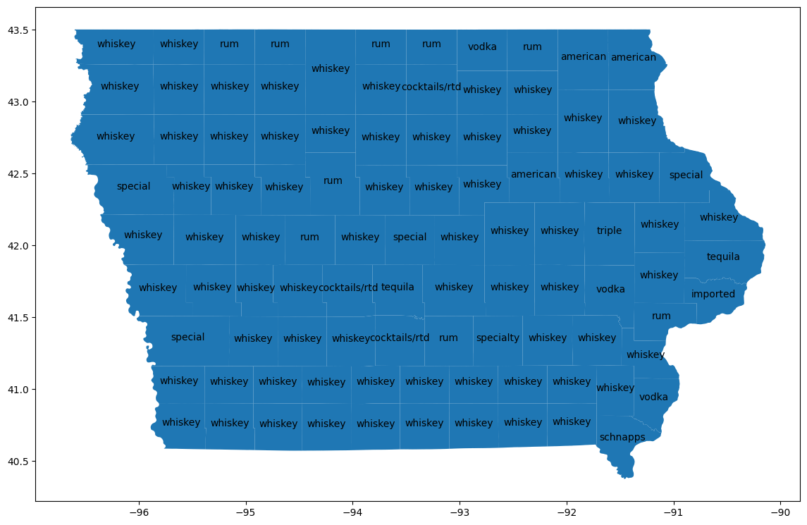
카운티 시각화
bigquery-public-data.geo_us_boundaries.counties 테이블과 조인하여 각 카운티의 지리적 영역을 가져옵니다. 카운티 이름은 미국 전역에서 고유하지 않으므로 아이오와주의 카운티만 포함하도록 필터링합니다. 아이오와의 FIPS 코드는 '19'입니다.
counties_geo = (
    bpd.read_gbq("bigquery-public-data.geo_us_boundaries.counties")
    .assign(county=lambda _: _['county_name'].str.upper())
)
counties_plus = (
    counties
    .reset_index(drop=False)
    .merge(counties_geo[counties_geo['state_fips_code'] == '19'], on="county", how="left")
    .dropna(subset=["county_geom"])
    .to_pandas()
)
counties_plus
예상 출력:
county	lemma	cohens_h	cohens_h_int	geo_id	state_fips_code	...
0	ALLAMAKEE	american	0.087931	87930	19005	19	...
1	BLACK HAWK	american	0.106256	106256	19013	19	...
2	WINNESHIEK	american	0.093101	93101	19191	19	...
...	...	...	...	...	...	...	...	...	...	...	...	...	...	...	...	...	...	...	...	...	...
96	CLINTON	tequila	0.075708	75707	19045	19	...
97	POLK	tequila	0.087438	87438	19153	19	...
98	LEE	schnapps	0.064663	64663	19111	19	...
99 rows × 23 columns
GeoPandas를 사용하여 지도에서 이러한 차이를 시각화합니다.
import geopandas

counties_plus = geopandas.GeoDataFrame(counties_plus, geometry="county_geom")

# https://stackoverflow.com/a/42214156/101923
ax = counties_plus.plot(figsize=(14, 14))
counties_plus.apply(
    lambda row: ax.annotate(
        text=row['lemma'],
        xy=row['county_geom'].centroid.coords[0],
        ha='center'
    ),
    axis=1,
)
9. 삭제
이 튜토리얼을 위해 새 Google Cloud 프로젝트를 만든 경우 삭제하여 테이블 또는 기타 생성된 리소스에 대한 추가 요금을 방지할 수 있습니다.
또는 이 튜토리얼에서 만든 Cloud 함수, 서비스 계정, 데이터 세트를 삭제합니다.
10. 축하합니다.
BigQuery DataFrames를 사용하여 구조화된 데이터를 정리하고 분석했습니다. 이 과정에서 Google Cloud의 공개 데이터 세트, BigQuery Studio의 Python 노트북, BigQuery ML, BigQuery 원격 함수, BigQuery DataFrames의 강력한 기능을 살펴봤습니다. 앞으로의 활동이 더욱 기대됩니다.
다음 단계
- 미국 이름 데이터베이스와 같은 다른 데이터에도 이 단계를 적용합니다.
- 노트북에서 Python 코드를 생성해 보세요. BigQuery Studio의 Python 노트북은 Colab Enterprise에서 제공합니다. 힌트: 테스트 데이터 생성에 대한 도움을 요청하는 것이 매우 유용합니다.
- GitHub에서 BigQuery DataFrames 샘플 노트북을 살펴봅니다.
- BigQuery Studio에서 노트북을 실행하는 일정을 만듭니다.
- BigQuery DataFrames를 사용하여 원격 함수를 배포하여 서드 파티 Python 패키지를 BigQuery와 통합합니다.