Effortless Data Prep in BigQuery: A Low-Coder's Guide

1. Introduction

Data analysts are often faced with valuable data locked in semi-structured formats like JSON payloads. Extracting and preparing this data for analysis and machine learning has traditionally been a significant technical hurdle, traditionally requiring complex ETL scripts and the intervention of a data engineering team.

This codelab provides a technical blueprint for data analysts to overcome this challenge independently. It demonstrates a "low-code" approach to building an end-to-end AI pipeline. You will learn how to go from a raw CSV file in Google Cloud Storage to powering an AI-driven recommendation feature, using only the tools available within the BigQuery Studio.

The primary objective is to demonstrate a robust, fast, and analyst-friendly workflow that moves beyond complex, code-heavy processes to generate real business value from your data.

Prerequisites

A basic understanding of the Google Cloud Console
Basic skills in command line interface and Google Cloud Shell

What you'll learn

How to ingest and transform a CSV file directly from Google Cloud Storage using BigQuery Data Preparation.
How to use no-code transformations to parse and flatten nested JSON strings within your data.
How to create a BigQuery ML remote model that connects to a Vertex AI foundation model for text embedding.
How to use the ML.GENERATE_TEXT_EMBEDDING function to convert textual data into numerical vectors.
How to use the ML.DISTANCE function to calculate cosine similarity and find the most similar items in your dataset.

What you'll need

A Google Cloud Account and Google Cloud Project
A web browser such as Chrome

Key concepts

BigQuery Data preparation: A tool within BigQuery Studio that provides an interactive, visual interface for data cleaning and preparation. It suggests transformations and allows users to build data pipelines with minimal code.
BQML Remote Model: A BigQuery ML object that acts as a proxy to a model hosted on Vertex AI (like Gemini). It allows you to invoke powerful, pre-trained AI models using familiar SQL syntax.
Vector embedding: A numerical representation of data, such as text or images. In this codelab, we'll convert text descriptions of artwork into vectors, where similar descriptions result in vectors that are "closer" together in multi-dimensional space.
Cosine similarity: A mathematical measure used to determine how similar two vectors are. It's the core of our recommendation engine's logic, used by the ML.DISTANCE function to find the "closest" (most similar) artworks.

2. Setup and requirements

Start Cloud Shell

While Google Cloud can be operated remotely from your laptop, in this codelab you will be using Google Cloud Shell, a command line environment running in the Cloud.

From the Google Cloud Console, click the Cloud Shell icon on the top right toolbar:

It should only take a few moments to provision and connect to the environment. When it is finished, you should see something like this:

This virtual machine is loaded with all the development tools you'll need. It offers a persistent 5GB home directory, and runs on Google Cloud, greatly enhancing network performance and authentication. All of your work in this codelab can be done within a browser. You do not need to install anything.

Enable required APIs and configure environment

Inside Cloud Shell, run the following commands to set your project ID, define environment variables, and enable all the necessary APIs for this codelab.

export PROJECT_ID=$(gcloud config get-value project)
gcloud config set project $PROJECT_ID
export LOCATION="US"
export GCS_BUCKET_NAME="met-artworks-source-${PROJECT_ID}" # Must be a globally unique name

gcloud services enable bigquery.googleapis.com \
                       storage.googleapis.com \
                       aiplatform.googleapis.com \
                       bigqueryconnection.googleapis.com

Create a BigQuery dataset and a GCS Bucket

Create a new BigQuery dataset to house our tables and a Google Cloud Storage bucket to store our source CSV file.

# Create the BigQuery Dataset in the US multi-region
bq --location=$LOCATION mk --dataset $PROJECT_ID:met_art_dataset

# Create the GCS Bucket
gcloud storage buckets create gs://$GCS_BUCKET_NAME --project=$PROJECT_ID --location=$LOCATION

Prepare and Upload the Sample Data

Clone the GitHub repository containing the sample CSV file and then upload it to the GCS bucket you just created.

# Clone the repository
git clone https://github.com/GoogleCloudPlatform/devrel-demos.git

# Navigate to the correct directory
cd devrel-demos/data-analytics/dataprep

# Upload the CSV file to your GCS bucket
gsutil cp dataprep-met-bqml.csv gs://$GCS_BUCKET_NAME/

3. From GCS to BigQuery with Data preparation

In this section, we will use a visual, no-code interface to ingest our CSV file from GCS, clean it, and load it into a new BigQuery table.

Launch Data Preparation and Connect to the Source

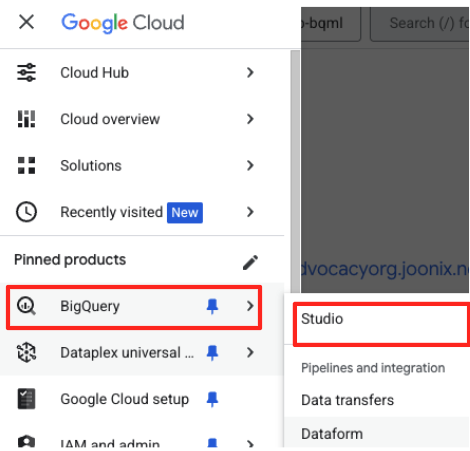
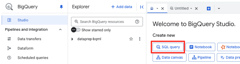
In the Google Cloud Console, navigate to the BigQuery Studio.

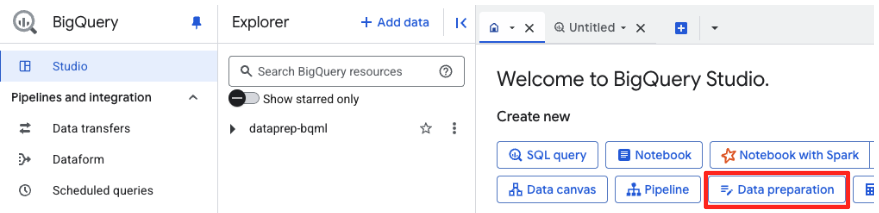
In the welcome page, click the Data preparation card to begin.

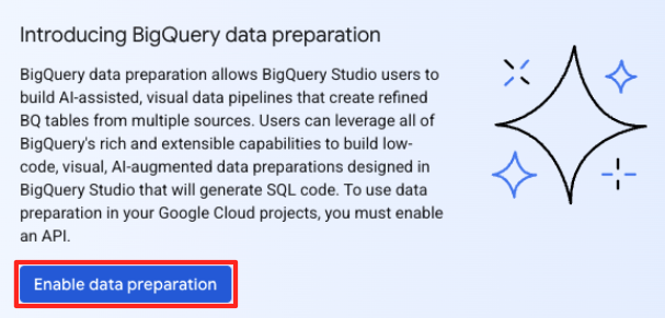
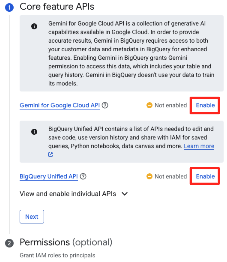
If this is your first time, you may need to enable required APIs. Click Enable for both the "Gemini for Google Cloud API" and the "BigQuery Unified API". Once they are enabled, you can close this panel.

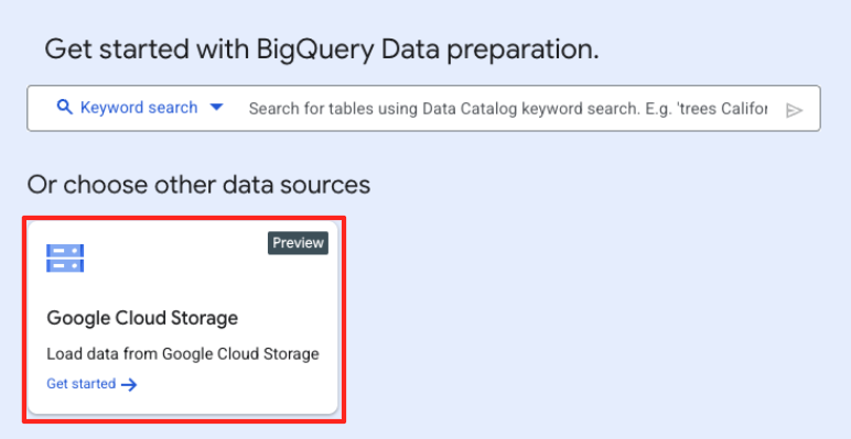
In the main Data preparation window, under "choose other data sources", click Google Cloud Storage. This will open the "Prepare data" panel on the right.

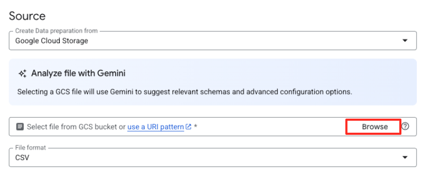
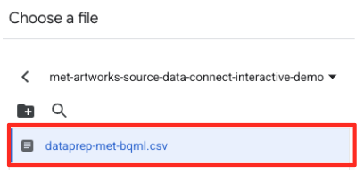
Click the Browse button to select your source file.

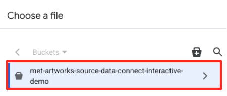
Navigate to the GCS bucket you created earlier (met-artworks-source-...) and select the dataprep-met-bqml.csv file. Click Select.

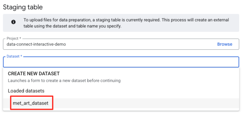
Next, you need to configure a staging table.
For Dataset, select the met_art_dataset you created.
For Table name, enter a name, for example, temp.
Click Create.

Transform and Clean the Data

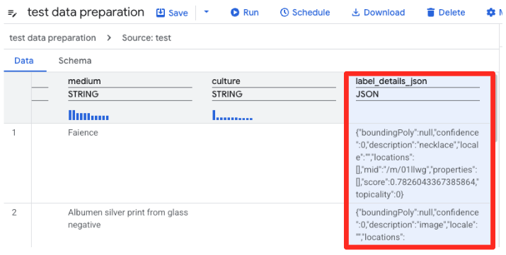
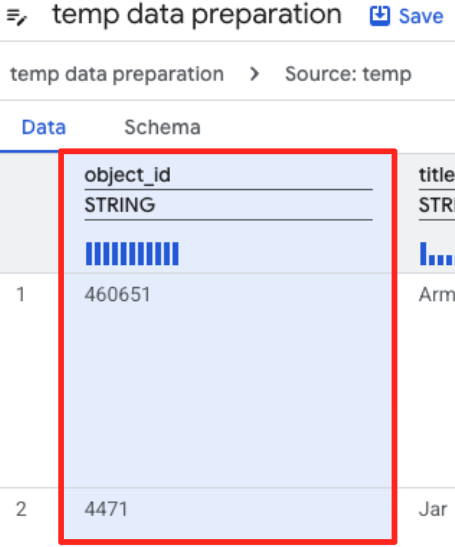
BigQuery's Data preparation will now load a preview of the CSV. Find the label_details_json column, which contains the long JSON string. Click on the column header to select it.

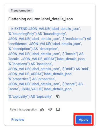
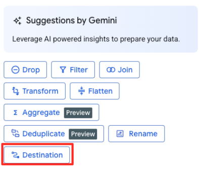
In the Suggestions panel on the right, Gemini in BigQuery will automatically suggest relevant transformations. Click the Apply button on the "Flattening column label_details_json" card. This will extract the nested fields (description, score, etc) into their own top-level columns.

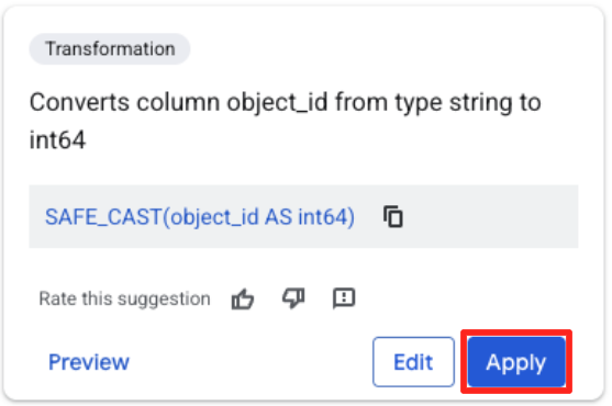
Click the object_id column, and click the apply button on the "Converts column object_id from type string to int64.

Define the Destination and Run the Job

In the right-hand panel, click the Destination button to configure the output of your transformation.

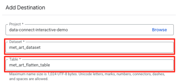
Set the destination details:
The Dataset should be pre-filled with met_art_dataset.
Enter a new Table name for the output: met_art_flatten_table.
Click Save.

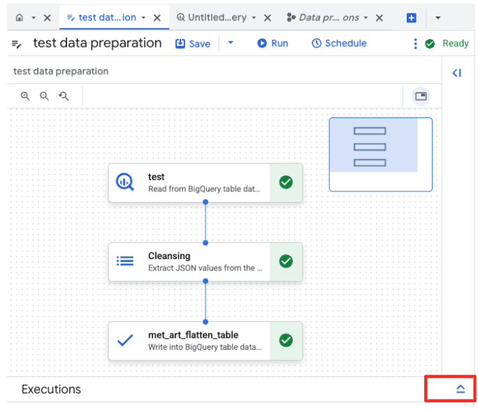
Click the Run button, and wait until the data preparation job is completed.

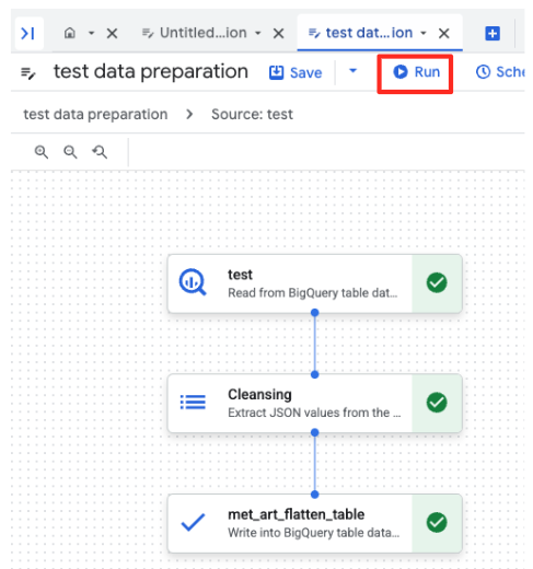
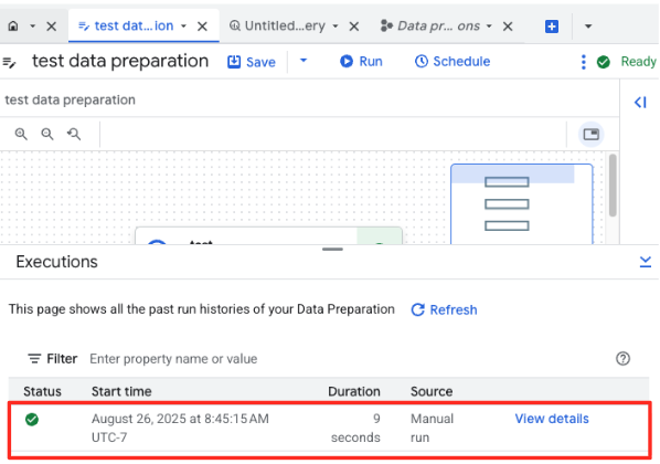
You can monitor the job's progress in the Executions tab at the bottom of the page. After a few moments, the job will complete.

4. Generating Vector Embeddings with BQML

Now that our data is clean and structured, we'll use BigQuery ML for the core AI task: converting the textual descriptions of the artwork into numerical vector embeddings.

Create a BigQuery Connection

To allow BigQuery to communicate with Vertex AI services, you must first create a BigQuery Connection.

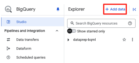
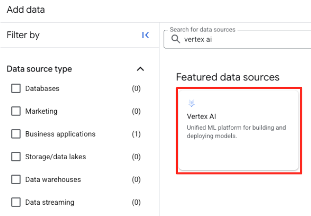
In the BigQuery Studio's Explorer panel, click the "+ Add data" button.

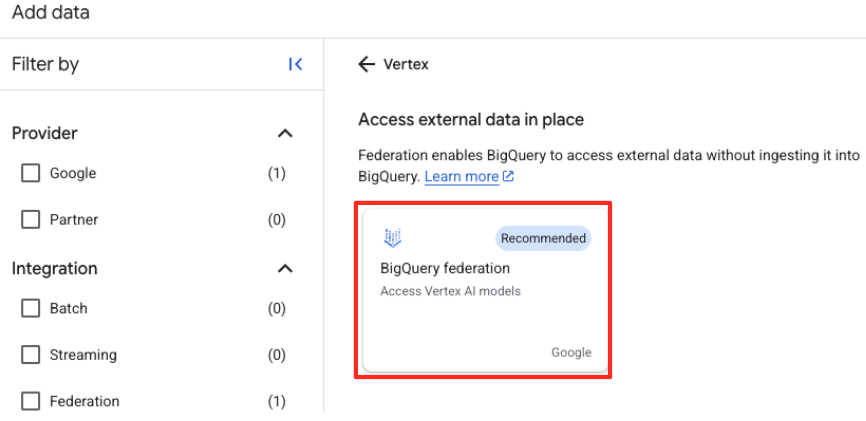
In the right-hand panel, use the search bar to type Vertex AI. Select it and then BigQuery federation from the filtered list.

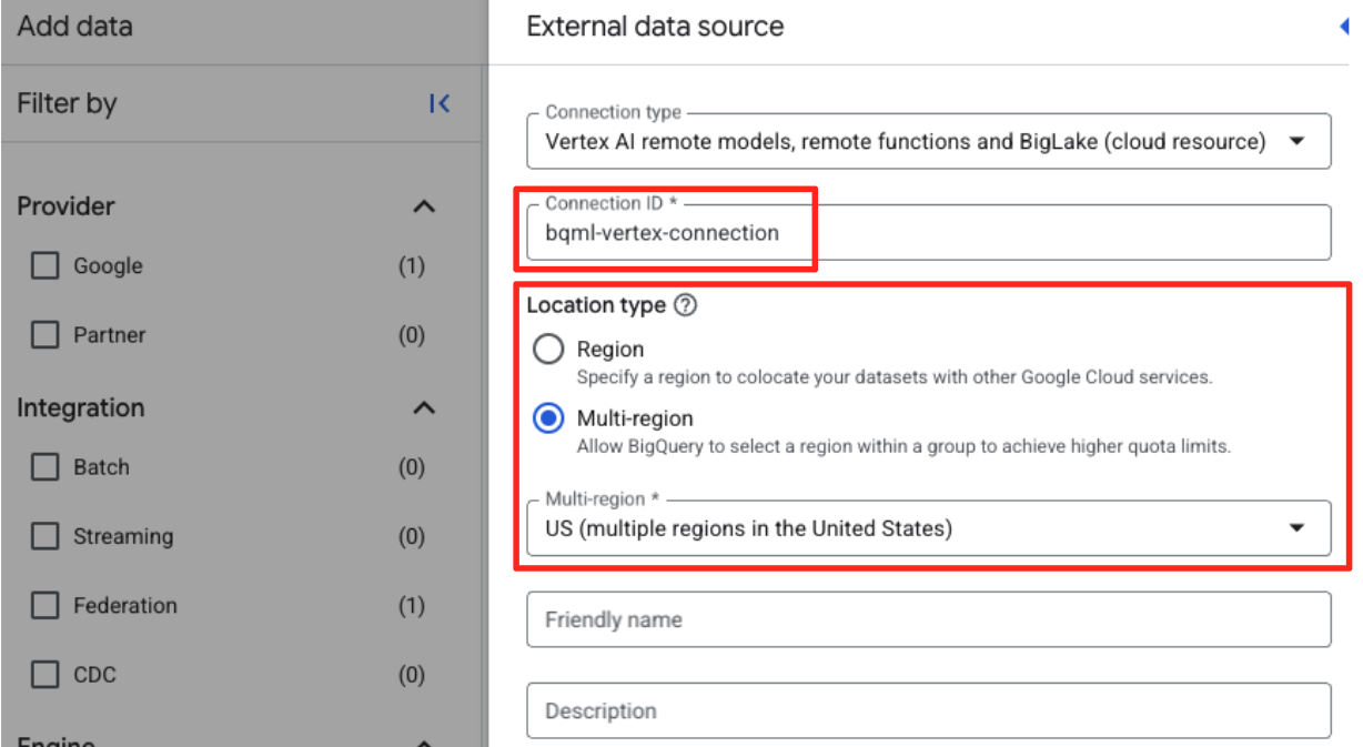
This will open the External data source form. Fill in the following details:

Connection ID: Enter the connection ID (e.g., bqml-vertex-connection)
Location Type: Ensure Multi-region is selected.
Location: Select the location (e.g., US).

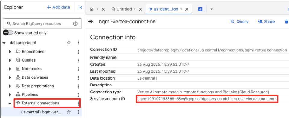
Once the connection is created, a confirmation dialog will appear. Click Go to Connection or External connections in the Explorer tab. On the connection details page, copy the full ID to your clipboard. This is the service account identity that BigQuery will use to call Vertex AI.

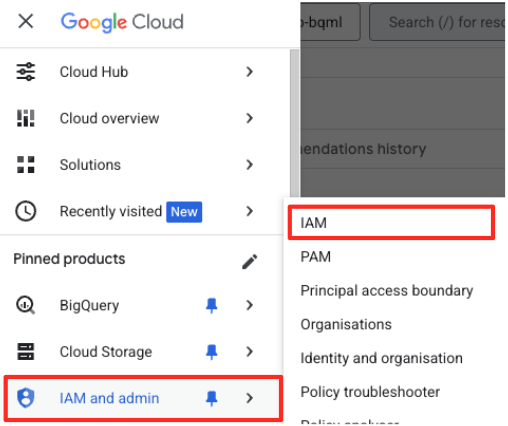
In the Google Cloud Console navigation menu, go to IAM & admin > IAM.

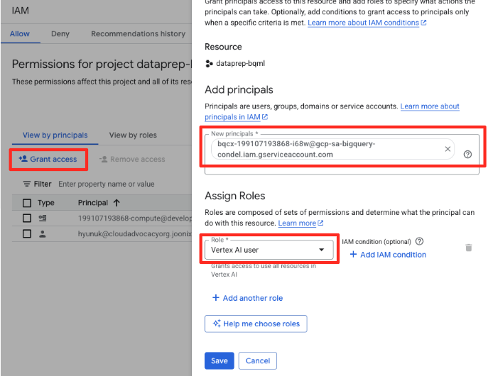
Click the "Grant access" button
Paste the service account you copied in the previous step in the New principals field.
Assign "Vertex AI user" at the Role dropdown, and click "Save".

This critical step ensures BigQuery has the proper authorization to use Vertex AI models on your behalf.

Create a Remote model

In the BigQuery Studio, open a new SQL editor tab. This is where you will define the BQML model that connects to Gemini.

This statement doesn't train a new model. It simply creates a reference in BigQuery that points to a powerful, pre-trained gemini-embedding-001 model using the connection you just authorized.

Copy the entire SQL script below and paste it into the BigQuery editor.

CREATE OR REPLACE MODEL `met_art_dataset.embedding_model`
REMOTE WITH CONNECTION `US.bqml-vertex-connection`
OPTIONS (endpoint = 'gemini-embedding-001');

Generate Embeddings

Now, we will use our BQML model to generate the vector embeddings. Instead of simply converting a single text label for each row, we will use a more sophisticated approach to create a richer, more meaningful "semantic summary" for each artwork. This will result in higher-quality embeddings and more accurate recommendations.

This query performs a critical preprocessing step:

It uses a WITH clause to first create a temporary table.
Inside it, we GROUP BY each object_id to combine all information about a single artwork into one row.
We use the STRING_AGG function to merge all the separate text descriptions (like ‘Portrait', ‘Woman', ‘Oil on canvas') into a single, comprehensive text string, ordering them by their relevance score.

This combined text gives the AI a much richer context about the artwork, leading to more nuanced and powerful vector embeddings.

In a new SQL editor tab, paste and run the following query:

CREATE OR REPLACE TABLE `met_art_dataset.artwork_embeddings` AS
WITH artwork_semantic_text AS (
  -- First, we group all text labels for each artwork into a single row.
  SELECT
    object_id,
    ANY_VALUE(title) AS title,
    ANY_VALUE(artist_display_name) AS artist_display_name,
    -- STRING_AGG combines all descriptions into one comma-separated string,
    -- ordering them by score to put the most relevant labels first.
    STRING_AGG(description, ', ' ORDER BY score DESC) AS aggregated_labels
  FROM
    `met_art_dataset.met_art_flatten_table`
  GROUP BY
    object_id
)
SELECT
  *
FROM ML.GENERATE_TEXT_EMBEDDING(
  MODEL `met_art_dataset.embedding_model`,
  (
    -- We pass the new, combined string as the content to be embedded.
    SELECT
      object_id,
      title,
      artist_display_name,
      aggregated_labels AS content
    FROM
      artwork_semantic_text
  )
);

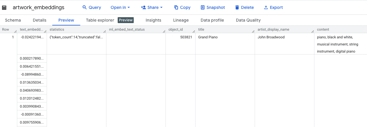
This query will take approximately 10 minutes. Once the query completes, verify the results. In the Explorer panel, find your new artwork_embeddings table and click on it. In the table schema viewer, you will see the object_id, the new ml_generate_text_embedding_result column containing the vectors, and also the aggregated_labels column that was used as the source text.

5. Finding Similar Artworks with SQL

With our high-quality, context-rich vector embeddings created, finding thematically similar artworks is as simple as running a SQL query. We use the ML.DISTANCE function to calculate the cosine similarity between vectors. Because our embeddings were generated from aggregated text, the similarity results will be more accurate and relevant.

In a new SQL editor tab, paste the following query. This query simulates the core logic of a recommendation application:

It first selects the vector for a single, specific artwork (in this case, Van Gogh's "Cypresses," which has an object_id of 436535).
It then calculates the distance between that single vector and all other vectors in the table.
Finally, it orders the results by distance (a smaller distance means more similar) to find the top 10 closest matches.

WITH selected_artwork AS (
  SELECT text_embedding
  FROM `met_art_dataset.artwork_embeddings`
  WHERE object_id = 436535
)
SELECT
  base.object_id,
  base.title,
  base.artist_display_name,
  -- ML.DISTANCE calculates the cosine distance between the two vectors.
  -- A smaller distance means the items are more similar.
  ML.DISTANCE(base.text_embedding, (SELECT text_embedding FROM selected_artwork), 'COSINE') AS similarity_distance
FROM
  `met_art_dataset.artwork_embeddings` AS base, selected_artwork
ORDER BY
  similarity_distance
LIMIT 10;

Run the query. The results will list object_ids, with the closest matches at the top. The source artwork will appear first with a distance of 0. This is the core logic that powers an AI recommendation engine, and you've built it entirely within BigQuery using just SQL.

6. (OPTIONAL) Running the demo in Cloud Shell

To bring the concepts from this codelab to life, the repository you cloned includes a simple web application. This optional demo uses the artwork_embeddings table you created to power a visual search engine, allowing you to see the AI-driven recommendations in action.

To run the demo in Cloud Shell, follow these steps:

Set Environment Variables: Before running the application, you need to set the PROJECT_ID and BIGQUERY_DATASET environment variables.

export PROJECT_ID=$(gcloud config get-value project)
export BIGQUERY_DATASET=met_art_dataset
export REGION='us-central1'
bq cp bigquery-public-data:the_met.images $PROJECT_ID:met_art_dataset.images

Install dependencies and start the backend server.

cd ~/devrel-demos/data-analytics/dataprep/backend/ && npm install
node server.js

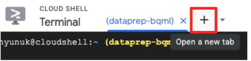
You will need a second terminal tab to run the frontend application. Click the "+" icon to open a new Cloud Shell tab.

Now, in the new tab, execute the following command to install dependencies and run the frontend server

cd ~/devrel-demos/data-analytics/dataprep/frontend/ && npm install
npm run dev

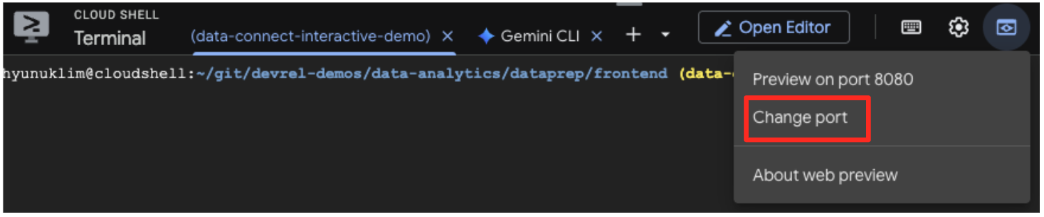
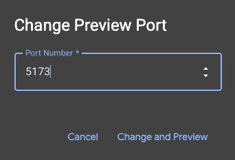
Preview the application: In the Cloud Shell toolbar, click on the Web Preview icon and select Preview on port 5173. This will open a new browser tab with the application running. You can now use the application to search for artworks and see the similarity search in action.

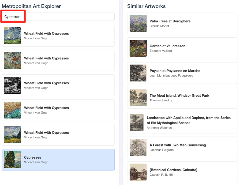
To connect this visual demo back to the work you did in BigQuery SQL editor, try typing "Cypresses" in the search bar. This is the same artwork(object_id=436535) you used in the ML.DISTANCE query. Then click on the Cypresses image when it appears in the left panel, you will observe the results on the right. The application displays the most similar artworks, visually demonstrating the power of the vector similarity search you built.

7. Cleaning up your environment

To avoid incurring future charges to your Google Cloud account for the resources used in this codelab, you should delete the resources you created.

Run the following commands in your Cloud Shell terminal to remove the service account, the BigQuery connection, the GCS Bucket, and the BigQuery dataset.

# Re-run these exports if your Cloud Shell session timed out
export PROJECT_ID=$(gcloud config get-value project)
export LOCATION="US"
export GCS_BUCKET_NAME="met-artworks-source-${PROJECT_ID}"
export BQ_CONNECTION_ID="bqml-vertex-connection"

Remove BigQuery Connection and GCS Bucket

# Delete the BigQuery connection
bq rm --connection $LOCATION.$BQ_CONNECTION_ID

# Delete the GCS bucket and its contents
gcloud storage rm --recursive gs://$GCS_BUCKET_NAME

Delete the BigQuery dataset

Finally, delete the BigQuery dataset. This command is irreversible. The -f (force) flag removes the dataset and all its tables without prompting for confirmation.

# Manually type this command to confirm you are deleting the correct dataset
bq rm -r -f --dataset $PROJECT_ID:met_art_dataset

8. Congratulations!

You have successfully built an end-to-end, AI-powered data pipeline.

You started with a raw CSV file in a GCS bucket, used BigQuery Data Prep's low-code interface to ingest and flatten complex JSON data, created a powerful BQML remote model to generate high-quality vector embeddings with a Gemini model, and executed a similarity search query to find related items.

You are now equipped with the fundamental pattern for building AI-assisted workflows on Google Cloud, transforming raw data into intelligent applications with speed and simplicity.

What's Next?

Visualize your results in Looker Studio: Connect your artwork_embeddings BigQuery table directly to Looker Studio (it's free!). You can build an interactive dashboard where users can select an artwork and see a visual gallery of the most similar pieces without writing any frontend code.
Automate with Scheduled Queries: You don't need a complex orchestration tool to keep your embeddings up-to-date. Use BigQuery's built-in Scheduled Queries feature to automatically re-run the ML.GENERATE_TEXT_EMBEDDING query on a daily or weekly basis.
Generate an app with the Gemini CLI: Use the Gemini CLI to generate a complete application simply by describing your requirement in plain text. This allows you to quickly build a working prototype for your similarity search without writing the Python code manually.
Read the documentation:
- Introduction to BigQuery data preparation
- Code Sample on GitHub