
关于此 Codelab
2. 设置
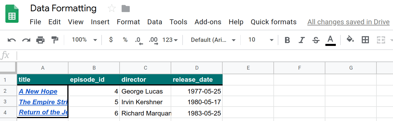
在继续操作之前,您需要一个包含一些数据的电子表格。和之前一样,我们提供了一个数据表,您可复制它来进行这些练习。请执行以下步骤:
- 点击此链接复制数据表,然后点击创建副本。新电子表格将放入您的 Google 云端硬盘文件夹,并命名为“数据格式设置的副本”。
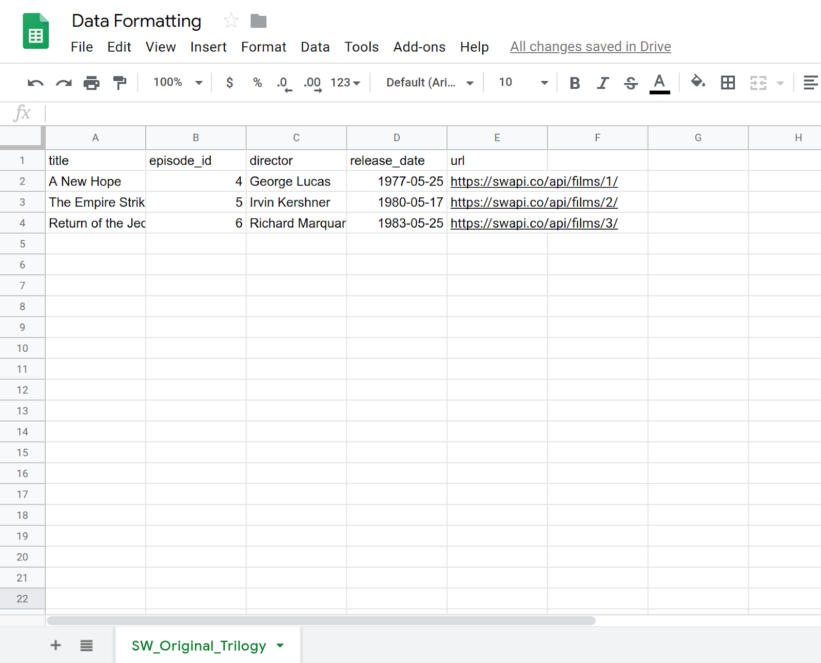
- 点击电子表格标题,将其从“数据格式设置的副本”更改为“数据格式设置”。您的工作表应如下所示,其中包含有关前三部《星球大战》电影的一些基本信息:
- 选择扩展 > Apps 脚本以打开脚本编辑器。
- 点击 Apps 脚本项目的标题,并将其从“未命名项目”更改为“数据格式设置”。点击重命名以保存标题更改。
使用此电子表格和项目后,您就可以启动 Codelab 了。请转到下一部分,开始了解 Apps 脚本中的基本格式设置。
3. 创建自定义菜单
您可以在 Apps 脚本中对您的 Google 表格应用几种基本的格式设置方法。以下练习介绍了几种设置数据格式的方法。为帮助您控制进行格式设置的操作,我们将创建一个包含所需菜单项的自定义菜单。处理数据 Codelab 中介绍了创建自定义菜单的流程,但本文将再次对此进行总结。
实现
让我们现在来创建自定义菜单。
- 在 Apps 脚本编辑器中,将脚本项目中的代码替换为以下代码:
/**
 * A special function that runs when the spreadsheet is opened
 * or reloaded, used to add a custom menu to the spreadsheet.
 */
function onOpen() {
  // Get the spreadsheet's user-interface object.
  var ui = SpreadsheetApp.getUi();

  // Create and add a named menu and its items to the menu bar.
  ui.createMenu('Quick formats')
   .addItem('Format row header', 'formatRowHeader')
   .addItem('Format column header', 'formatColumnHeader')
   .addItem('Format dataset', 'formatDataset')
  .addToUi();
}
- 保存脚本项目。
- 在脚本编辑器中,从函数列表中选择
onOpen,然后点击运行。这会运行onOpen()来重新构建电子表格菜单,因此您无需重新加载电子表格。
代码审核
我们来看看此代码,了解其工作原理。在 onOpen() 中,第一行使用 getUi() 方法获取 Ui 对象,该对象表示与该脚本绑定的活跃电子表格的界面。
接下来的几行代码会创建一个菜单 (Quick formats)、将一些菜单项(Format row header、Format column header 和 Format dataset)添加到该菜单中,然后将该菜单添加到电子表格的界面。这分别使用 createMenu(caption)、addItem(caption, functionName) 和 addToUi() 方法完成。
addItem(caption, functionName) 方法会在菜单项标签和 Apps 脚本函数之间创建关联,使得后者会在选中菜单项时运行。例如,选择 Format row header 菜单项会导致 Google 表格尝试运行 formatRowHeader() 函数(尚不存在)。
结果
在电子表格中,点击 Quick formats 菜单来查看新的菜单项:
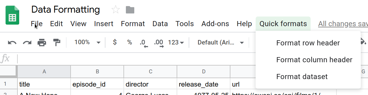
点击这些菜单项会导致错误,因为您尚未实现其相应的函数,所以我们稍后再执行该操作。
4. 设置标题行的格式
电子表格中的数据集通常包含标题行,用于标识每一列中的数据。建议您在为标题行设置格式时将它们与电子表格中的其他数据区分开来。
在第一个 Codelab 中,您为标题构建了宏并调整了其代码。在这里,您需要使用 Apps 脚本从头开始设置标题行的格式。您要创建的标题行会以粗体显示标题文字,将背景颜色设为深蓝绿色,将文字设为白色,并会添加一些实线边框。
实现
如需实现格式设置操作,您需要使用您之前用过的电子表格服务方法,但在这里您还需要使用该服务提供的一些格式设置方法。请按以下步骤操作:
- 在 Apps 脚本编辑器中,将以下函数添加到脚本项目的末尾:
/**
 * Formats top row of sheet using our header row style.
 */
function formatRowHeader() {
  // Get the current active sheet and the top row's range.
  var sheet = SpreadsheetApp.getActiveSheet();
  var headerRange = sheet.getRange(1, 1, 1, sheet.getLastColumn());

  // Apply each format to the top row: bold white text,
  // blue-green background, and a solid black border
  // around the cells.
  headerRange
    .setFontWeight('bold')
    .setFontColor('#ffffff')
    .setBackground('#007272')
    .setBorder(
      true, true, true, true, null, null,
      null,
      SpreadsheetApp.BorderStyle.SOLID_MEDIUM);

}
- 保存脚本项目。
代码审核
与许多格式设置任务一样,实现格式设置的 Apps 脚本代码也很简单。前两行代码会使用前面提到过的方法获取对当前活跃工作表 (sheet) 以及对工作表首行 (headerRange)) 的引用。Sheet.getRange(row, column, numRows, numColumns) 方法会指定首行,且仅包含那些包含数据的列。Sheet.getLastColumn() 方法会返回包含工作表数据的最后一列的列索引。在我们的示例中,该列为 E(网址)。
其余代码只是调用各种 Range 方法以将格式设置选项应用于 headerRange 中的所有单元格。为了便于阅读代码,我们使用方法链来依次调用每种格式设置方法:
Range.setFontWeight(fontWeight)用于将字体粗细设为粗体。Range.setFontColor(color)用于将字体颜色设为白色。Range.setBackground(color)用于将背景颜色设为深蓝绿色。setBorder(top, left, bottom, right, vertical, horizontal, color, style)会在指定范围的单元格周围显示实线黑色边框。
最后一个方法包含多个参数,下面我们来看看每个参数的作用。前四个参数(均设置为 true)用于告知 Apps 脚本在指定范围的上方、下方、左侧和右侧添加边框。第五个和第六个参数(null 和 null)用于指示 Apps 脚本避免在选定范围内更改任何边框线。第七个参数 (null) 用于指示边框的颜色应默认为黑色。最后一个参数则指定要使用的边框样式的类型,取自 SpreadsheetApp.BorderStyle 提供的选项。
结果
您可以执行以下操作来查看格式设置函数的实际效果:
- 如果您尚未保存脚本项目,请在 Apps 脚本编辑器中进行保存。
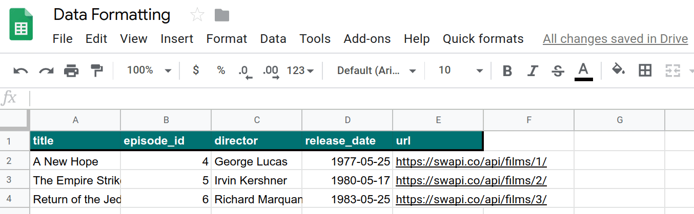
- 依次点击快速格式 > 设置行标题的格式菜单项。
结果应如下所示:
现在,您已自动执行该格式设置任务。下一部分会使用同样的方法来为列标题创建不同的格式样式。
5. 设置列标题的格式
如果您可以创建个性化的行标题,那么列标题也可以。好的列标题可以提高某些数据集的可读性。例如,该电子表格中的标题列可以通过以下格式选项进行改进:
- 将文本设置为粗体
- 将文本设置为斜体
- 添加单元格边框
- 使用网址列内容插入超链接。添加这些超链接后,您可以移除网址列来帮助清理工作表。
接下来,您将实现一个 formatColumnHeader() 函数,来将这些更改应用于工作表中的第一列。为使代码更易于阅读,我们还将实现两个辅助函数。
实现
与之前一样,您需要添加一个函数来自动设置列标题的格式。请按以下步骤操作:
- 在 Apps 脚本编辑器中,将以下
formatColumnHeader()函数添加到脚本项目的末尾:
/**
 * Formats the column header of the active sheet.
 */
function formatColumnHeader() {
  var sheet = SpreadsheetApp.getActiveSheet();

  // Get total number of rows in data range, not including
  // the header row.
  var numRows = sheet.getDataRange().getLastRow() - 1;

  // Get the range of the column header.
  var columnHeaderRange = sheet.getRange(2, 1, numRows, 1);

  // Apply text formatting and add borders.
  columnHeaderRange
    .setFontWeight('bold')
    .setFontStyle('italic')
    .setBorder(
      true, true, true, true, null, null,
      null,
      SpreadsheetApp.BorderStyle.SOLID_MEDIUM);

  // Call helper method to hyperlink the first column contents
  // to the url column contents.
  hyperlinkColumnHeaders_(columnHeaderRange, numRows);
}
- 将以下辅助函数添加到脚本项目末尾的
formatColumnHeader()函数之后:
/**
 * Helper function that hyperlinks the column header with the
 * 'url' column contents. The function then removes the column.
 *
 * @param {object} headerRange The range of the column header
 *   to update.
 * @param {number} numRows The size of the column header.
 */
function hyperlinkColumnHeaders_(headerRange, numRows) {
  // Get header and url column indices.
  var headerColIndex = 1;
  var urlColIndex = columnIndexOf_('url');

  // Exit if the url column is missing.
  if(urlColIndex == -1)
    return;

  // Get header and url cell values.
  var urlRange =
    headerRange.offset(0, urlColIndex - headerColIndex);
  var headerValues = headerRange.getValues();
  var urlValues = urlRange.getValues();

  // Updates header values to the hyperlinked header values.
  for(var row = 0; row < numRows; row++){
    headerValues[row][0] = '=HYPERLINK("' + urlValues[row]
      + '","' + headerValues[row] + '")';
  }
  headerRange.setValues(headerValues);

  // Delete the url column to clean up the sheet.
  SpreadsheetApp.getActiveSheet().deleteColumn(urlColIndex);
}

/**
 * Helper function that goes through the headers of all columns
 * and returns the index of the column with the specified name
 * in row 1. If a column with that name does not exist,
 * this function returns -1. If multiple columns have the same
 * name in row 1, the index of the first one discovered is
 * returned.
 *
 * @param {string} colName The name to find in the column
 *   headers.
 * @return The index of that column in the active sheet,
 *   or -1 if the name isn't found.
 */
function columnIndexOf_(colName) {
  // Get the current column names.
  var sheet = SpreadsheetApp.getActiveSheet();
  var columnHeaders =
    sheet.getRange(1, 1, 1, sheet.getLastColumn());
  var columnNames = columnHeaders.getValues();

  // Loops through every column and returns the column index
  // if the row 1 value of that column matches colName.
  for(var col = 1; col <= columnNames[0].length; col++)
  {
    if(columnNames[0][col-1] === colName)
      return col;
  }

  // Returns -1 if a column named colName does not exist.
  return -1;
}
- 保存脚本项目。
代码审核
下面分别介绍这三个函数中的代码:
formatColumnHeader()
正如您可能所需,此函数的前几行设置引用了我们感兴趣的工作表和范围的前几行:
- 活动工作表存储在
sheet中。 - 列标题中的行数会计算并保存在
numRows中。这里的代码会减去 1,因此行数不包括列标题:title。 - 列标题覆盖的范围存储在
columnHeaderRange中。
之后,代码会对列标题范围应用边框和粗体,就像在 formatRowHeader() 中一样。其中,Range.setFontStyle(fontStyle) 还可用于将文字设为斜体。
将超链接添加到标题列的操作会更为复杂,因此 formatColumnHeader() 会调用 hyperlinkColumnHeaders_(headerRange, numRows) 来执行该任务。这有助于保持代码简洁易读。
hyperlinkColumnHeaders_(headerRange, numRows)
该辅助函数首先识别标题的列索引(假设为索引 1)和 url 列。它会调用 columnIndexOf_('url') 来获取网址列的索引。如果未找到 url 列,该方法将退出且不会修改任何数据。
该函数会获取一个新范围 (urlRange),该范围将涵盖与标题列的各行所对应的网址。这是通过 Range.offset(rowOffset, columnOffset) 方法实现的,该方法可确保两个范围的大小相同。之后,系统将检索 headerColumn 和 url 列中的值(headerValues 和 urlValues)。
接下来,该函数会遍历每个列标题单元格的值,并将其替换为使用标题和 url 列内容构造的 Google 表格公式 =HYPERLINK()。之后,系统会使用 Range.setValues(values) 将修改后的标题值插入到工作表中。
最后,为帮助保持工作表整洁并消除冗余信息,我们会调用 Sheet.deleteColumn(columnPosition) 来移除 url 列。
columnIndexOf_(colName)
该辅助函数是一个简单的实用函数,它会在工作表的第一行中搜索特定名称。前三行代码使用您之前用过的方法从电子表格的第 1 行获取列标题名称的列表。这些名称存储在变量 columnNames 中。
之后,该函数会按顺序检查每个名称。如果找到与所搜索的名称相匹配的项,则会停止并返回相应列的索引。如果直至名称列表的末尾仍然找不到所搜索的名称,则会返回 -1,表示未找到该名称。
结果
您可以执行以下操作来查看格式设置函数的实际效果:
- 如果您尚未保存脚本项目,请在 Apps 脚本编辑器中进行保存。
- 依次点击快速格式 > 设置列标题的格式菜单项。
结果应如下所示:
现在,您已自动执行另一项格式设置任务。现在您已设置列标题和行标题的格式,下一部分将介绍如何设置数据的格式。
6. 设置数据集的格式
现在您已拥有标题,接下来我们将创建一个函数,用于设置工作表中其余数据的格式。我们将使用以下格式设置选项:
- 交替行背景颜色(称为条带)
- 更改日期格式
- 应用边框
- 自动调整所有列和行的大小
现在,您将创建一个 formatDataset() 函数和一个额外的辅助方法,来将这些格式应用于工作表数据。
实现
与前面一样,添加用于自动设置数据格式的函数。请按以下步骤操作:
- 在 Apps 脚本编辑器中,将以下
formatDataset()函数添加到脚本项目的末尾:
/**
 * Formats the sheet data, excluding the header row and column.
 * Applies the border and banding, formats the 'release_date'
 * column, and autosizes the columns and rows.
 */
function formatDataset() {
  // Get the active sheet and data range.
  var sheet = SpreadsheetApp.getActiveSheet();
  var fullDataRange = sheet.getDataRange();

  // Apply row banding to the data, excluding the header
  // row and column. Only apply the banding if the range
  // doesn't already have banding set.
  var noHeadersRange = fullDataRange.offset(
    1, 1,
    fullDataRange.getNumRows() - 1,
    fullDataRange.getNumColumns() - 1);

  if (! noHeadersRange.getBandings()[0]) {
    // The range doesn't already have banding, so it's
    // safe to apply it.
    noHeadersRange.applyRowBanding(
      SpreadsheetApp.BandingTheme.LIGHT_GREY,
      false, false);
  }

  // Call a helper function to apply date formatting
  // to the column labeled 'release_date'.
  formatDates_( columnIndexOf_('release_date') );

  // Set a border around all the data, and resize the
  // columns and rows to fit.
  fullDataRange.setBorder(
    true, true, true, true, null, null,
    null,
    SpreadsheetApp.BorderStyle.SOLID_MEDIUM);

  sheet.autoResizeColumns(1, fullDataRange.getNumColumns());
  sheet.autoResizeRows(1, fullDataRange.getNumRows());
}
- 在脚本项目末尾的
formatDataset()函数之后添加以下辅助函数:
/**
 * Helper method that applies a
 * "Month Day, Year (Day of Week)" date format to the
 * indicated column in the active sheet.
 *
 * @param {number} colIndex The index of the column
 *   to format.
 */
function formatDates_(colIndex) {
  // Exit if the given column index is -1, indicating
  // the column to format isn't present in the sheet.
  if (colIndex < 0)
    return;

  // Set the date format for the date column, excluding
  // the header row.
  var sheet = SpreadsheetApp.getActiveSheet();
  sheet.getRange(2, colIndex, sheet.getLastRow() - 1, 1)
    .setNumberFormat("mmmm dd, yyyy (dddd)");
}
- 保存脚本项目。
代码审核
下面分别介绍这两个函数中的代码:
formatDataset()
此函数采用的方法与您之前已实现的格式函数类似。首先,它会使用变量来保存对活跃工作表 (sheet) 和数据范围 (fullDataRange) 的引用。
之后,它会使用 Range.offset(rowOffset, columnOffset, numRows, numColumns) 方法创建一个范围 (noHeadersRange),以涵盖工作表中的所有数据(不包括列标题和行标题)。接下来,代码会验证此新范围是否已显示有条带(使用 Range.getBandings())。该验证是有必要的,因为如果您在已有条带的情况下尝试应用新的条带,Apps 脚本会抛出错误。如果条带不存在,该函数会使用 Range.applyRowBanding(bandingTheme, showHeader, showFooter) 添加浅灰色条带。否则,该函数会继续执行。
下一步会调用 formatDates_(colIndex) 辅助函数来设置“release_date”列中日期的格式(如下文所述)。该列是使用您之前实现的 columnIndexOf_(colName) 辅助函数指定的。
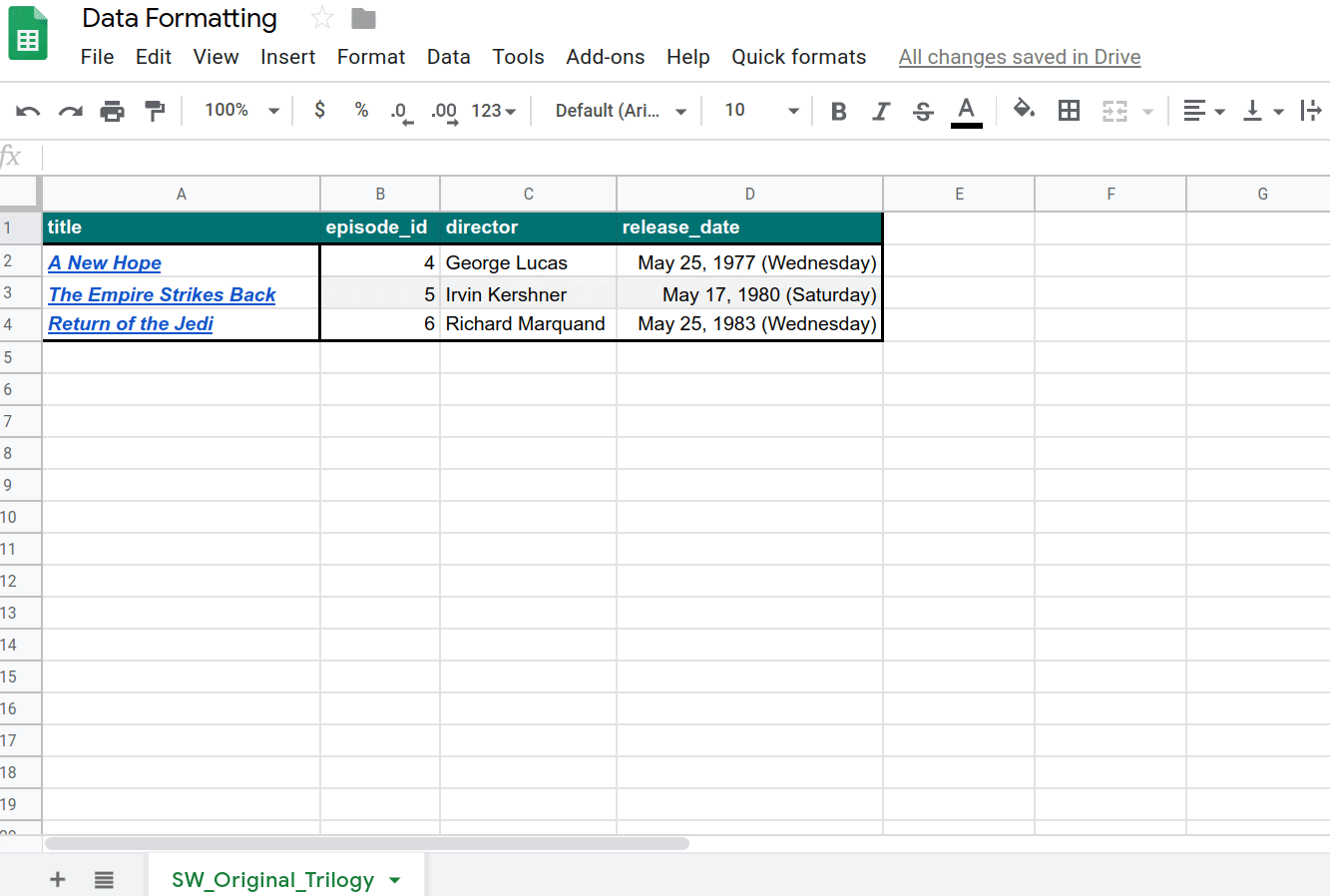
最后,通过添加其他边界框(如前所述)完成格式设置,并使用 Sheet.autoResizeColumns(columnPosition) 和 Sheet.autoResizeColumns(columnPosition) 方法更新。
formatDates_(colIndex)
该辅助函数使用提供的列索引将特定日期格式应用于相应列。具体而言,它会将日期值的格式设置为“月日,年(周几)”。
首先,该函数会验证提供的列索引是否有效(即不小于 0)。如果无效,它将直接返回而不执行任何操作。此检查可防止在工作表不包含“release_date”列时可能会导致的错误。
验证列索引后,该函数会获取覆盖该列的范围(不包括其标题行),并使用 Range.setNumberFormat(numberFormat) 来应用格式设置。
结果
您可以执行以下操作来查看格式设置函数的实际效果:
- 如果您尚未保存脚本项目,请在 Apps 脚本编辑器中进行保存。
- 依次点击快速格式 > 设置数据集的格式菜单项。
结果应如下所示:
您已自动执行另一项格式设置任务。现在,您已经有了这些格式设置命令,接下来我们将添加更多数据来应用这些命令。
7. 获取 API 数据并设置其格式
到目前为止,您已通过本 Codelab 了解了如何将 Apps 脚本用作一个替代方法来设置电子表格的格式。接下来,您需要编写代码来从公共 API 中提取数据,将数据插入电子表格,并设置数据格式来使其简洁易读。
在上一个 Codelab 中,您学习了如何从 API 中提取数据。在这里您将使用相同的方法。在本练习中,我们将使用公开提供的 Star Wars API (SWAPI) 来填充您的电子表格。具体而言,您将使用该 API 获取原始三部《星球大战》电影中出现的主要角色的相关信息。
您的代码将调用 API 以获取大量 JSON 数据,解析响应,将数据放在新工作表中,然后设置工作表的格式。
实现
在本部分中,您将添加一些额外的菜单项。每个菜单项都会调用一个封装容器脚本,将菜单项特定的变量传递给主函数 (createResourceSheet_())。接下来,您将实现该函数,以及另外三个辅助函数。与前面一样,这些辅助函数会帮助隔离任务的各个逻辑部分,并帮助保持代码简洁易读。
请执行以下操作:
- 在 Apps 脚本编辑器中,更新脚本项目中的
onOpen()函数以匹配以下内容:
/**
 * A special function that runs when the spreadsheet is opened
 * or reloaded, used to add a custom menu to the spreadsheet.
 */
function onOpen() {
  // Get the Ui object.
  var ui = SpreadsheetApp.getUi();

  // Create and add a named menu and its items to the menu bar.
  ui.createMenu('Quick formats')
    .addItem('Format row header', 'formatRowHeader')
    .addItem('Format column header', 'formatColumnHeader')
    .addItem('Format dataset', 'formatDataset')
    .addSeparator()
    .addSubMenu(ui.createMenu('Create character sheet')
                .addItem('Episode IV', 'createPeopleSheetIV')
                .addItem('Episode V', 'createPeopleSheetV')
                .addItem('Episode VI', 'createPeopleSheetVI')
                )
    .addToUi();
}
- 保存脚本项目。
- 在脚本编辑器中,从函数列表中选择
onOpen,然后点击运行。这会运行onOpen()以使用您添加的新选项重新构建电子表格菜单。 - 如需创建 Apps 脚本文件,请点击文件旁边的“添加文件”图标
 > 脚本。
> 脚本。 - 将新脚本命名为“API”,然后按 Enter 键。(Apps 脚本会自动将
.gs扩展名附加到脚本文件名中。) - 将新的 API.gs 文件中的代码替换为以下内容:
/**
 * Wrapper function that passes arguments to create a
 * resource sheet describing the characters from Episode IV.
 */
function createPeopleSheetIV() {
  createResourceSheet_('characters', 1, "IV");
}

/**
 * Wrapper function that passes arguments to create a
 * resource sheet describing the characters from Episode V.
 */
function createPeopleSheetV() {
  createResourceSheet_('characters', 2, "V");
}

/**
 * Wrapper function that passes arguments to create a
 * resource sheet describing the characters from Episode VI.
 */
function createPeopleSheetVI() {
  createResourceSheet_('characters', 3, "VI");
}

/**
 * Creates a formatted sheet filled with user-specified
 * information from the Star Wars API. If the sheet with
 * this data exists, the sheet is overwritten with the API
 * information.
 *
 * @param {string} resourceType The type of resource.
 * @param {number} idNumber The identification number of the film.
 * @param {number} episodeNumber The Star Wars film episode number.
 *   This is only used in the sheet name.
 */
function createResourceSheet_(
    resourceType, idNumber, episodeNumber) {

  // Fetch the basic film data from the API.
  var filmData = fetchApiResourceObject_(
      "https://swapi.dev/api/films/" + idNumber);

  // Extract the API URLs for each resource so the code can
  // call the API to get more data about each individually.
  var resourceUrls = filmData[resourceType];

  // Fetch each resource from the API individually and push
  // them into a new object list.
  var resourceDataList = [];
  for(var i = 0; i < resourceUrls.length; i++){
    resourceDataList.push(
      fetchApiResourceObject_(resourceUrls[i])
    );
  }

  // Get the keys used to reference each part of data within
  // the resources. The keys are assumed to be identical for
  // each object since they're all the same resource type.
  var resourceObjectKeys = Object.keys(resourceDataList[0]);

  // Create the sheet with the appropriate name. It
  // automatically becomes the active sheet when it's created.
  var resourceSheet = createNewSheet_(
      "Episode " + episodeNumber + " " + resourceType);

  // Add the API data to the new sheet, using each object
  // key as a column header.
  fillSheetWithData_(resourceSheet, resourceObjectKeys, resourceDataList);

  // Format the new sheet using the same styles the
  // 'Quick Formats' menu items apply. These methods all
  // act on the active sheet, which is the one just created.
  formatRowHeader();
  formatColumnHeader();
  formatDataset();

}
- 将以下辅助函数添加到 API.gs 脚本项目文件的末尾:
/**
 * Helper function that retrieves a JSON object containing a
 * response from a public API.
 *
 * @param {string} url The URL of the API object being fetched.
 * @return {object} resourceObject The JSON object fetched
 *   from the URL request to the API.
 */
function fetchApiResourceObject_(url) {
  // Make request to API and get response.
  var response =
    UrlFetchApp.fetch(url, {'muteHttpExceptions': true});

  // Parse and return the response as a JSON object.
  var json = response.getContentText();
  var responseObject = JSON.parse(json);
  return responseObject;
}

/**
 * Helper function that creates a sheet or returns an existing
 * sheet with the same name.
 *
 * @param {string} name The name of the sheet.
 * @return {object} The created or existing sheet
 *   of the same name. This sheet becomes active.
 */
function createNewSheet_(name) {
  var ss = SpreadsheetApp.getActiveSpreadsheet();

  // Returns an existing sheet if it has the specified
  // name. Activates the sheet before returning.
  var sheet = ss.getSheetByName(name);
  if (sheet) {
    return sheet.activate();
  }

  // Otherwise it makes a sheet, set its name, and returns it.
  // New sheets created this way automatically become the active
  // sheet.
  sheet = ss.insertSheet(name);
  return sheet;
}

/**
 * Helper function that adds API data to the sheet.
 * Each object key is used as a column header in the new sheet.
 *
 * @param {object} resourceSheet The sheet object being modified.
 * @param {object} objectKeys The list of keys for the resources.
 * @param {object} resourceDataList The list of API
 *   resource objects containing data to add to the sheet.
 */
function fillSheetWithData_(
    resourceSheet, objectKeys, resourceDataList) {
  // Set the dimensions of the data range being added to the sheet.
  var numRows = resourceDataList.length;
  var numColumns = objectKeys.length;

  // Get the resource range and associated values array. Add an
  // extra row for the column headers.
  var resourceRange =
    resourceSheet.getRange(1, 1, numRows + 1, numColumns);
  var resourceValues = resourceRange.getValues();

  // Loop over each key value and resource, extracting data to
  // place in the 2D resourceValues array.
  for (var column = 0; column < numColumns; column++) {

    // Set the column header.
    var columnHeader = objectKeys[column];
    resourceValues[0][column] = columnHeader;

    // Read and set each row in this column.
    for (var row = 1; row < numRows + 1; row++) {
      var resource = resourceDataList[row - 1];
      var value = resource[columnHeader];
      resourceValues[row][column] = value;
    }
  }

  // Remove any existing data in the sheet and set the new values.
  resourceSheet.clear()
  resourceRange.setValues(resourceValues);
}
- 保存脚本项目。
代码审核
您刚刚添加了大量代码。下面,我们来分别了解一下每个函数的工作原理:
onOpen()
在这里,您已经向 Quick formats 菜单添加了几个菜单项。您设置了分隔符行,然后使用 Menu.addSubMenu(menu) 方法创建了一个包含三个新菜单项的嵌套菜单结构。这些新菜单项是使用 Menu.addItem(caption, functionName) 方法添加的。
封装容器函数
添加的所有菜单项均执行类似操作:它们均尝试使用从 SWAPI 中提取的数据创建工作表。唯一的区别是它们侧重的影片不同。
比较简便的方法是编写一个函数来创建工作表,并通过让函数接受参数来确定要使用的影片。不过,Menu.addItem(caption, functionName) 方法不允许通过菜单调用来向其传递参数。那么,如何避免将同一代码编写三次呢?
答案是使用封装容器函数。封装容器函数属于轻量级函数,您可以在调用该函数后,立即调用另一个设置了特定参数的函数。
在这里,代码会使用三个封装容器函数:createPeopleSheetIV()、createPeopleSheetV() 和 createPeopleSheetVI()。菜单项会与这些函数相关联。当用户点击某个菜单项时,封装容器函数便会执行并立即调用主工作表构建器函数 createResourceSheet_(resourceType, idNumber, episodeNumber),并传递该菜单项所对应的参数。在这种情况下,意味着系统会指示工作表构建器函数创建一个工作表并填充某一部《星球大战》电影中的主要角色数据。
createResourceSheet_(resourceType, idNumber, episodeNumber)
这是本练习中使用的主工作表构建器函数。该函数会通过一些辅助函数来获取 API 数据,对数据进行解析,创建一个工作表并将 API 数据写入该工作表,然后使用您在前面部分构建的函数设置该工作表的格式。下面,我们来详细了解一下该流程:
首先,该函数会使用 fetchApiResourceObject_(url) 发出 API 请求,以检索基本电影信息。该 API 响应包含一系列网址,代码可以通过它们从影片中获取有关特定角色(此处称为资源)的更多详细信息。代码会将这些信息全部收集到 resourceUrls 数组中。
接下来,代码会反复使用 fetchApiResourceObject_(url) 针对 resourceUrls 中的每个资源网址调用该 API。结果存储在 resourceDataList 数组中。此数组的每个元素都是一个描述电影中不同角色的对象。
资源数据对象具有几个通用键,它们会映射到相应角色的相关信息。例如,键“name”会映射到电影中的角色名称。我们假定每个资源数据对象的键都完全相同,因为它们会使用通用的对象结构。由于后面需要用到键列表,因此代码会使用 JavaScript Object.keys() 方法将键列表存储在 resourceObjectKeys 中。
接下来,构建器函数会调用 createNewSheet_(name) 辅助函数来创建要在其中放置新数据的工作表。调用该辅助函数也会激活新工作表。
创建表格后,系统会调用辅助函数 fillSheetWithData_(resourceSheet, objectKeys, resourceDataList) 来将所有 API 数据添加到该工作表。
最后,系统将调用您之前构建的所有格式设置函数,对新数据应用相同的格式设置规则。由于新工作表处于活跃状态,因此代码可以重复使用这些函数而无需进行任何修改。
fetchApiResourceObject_(url)
该辅助函数类似于上一个 Codelab 处理数据中使用的 fetchBookData_(ISBN) 辅助函数。它会接受给定网址,并使用 UrlFetchApp.fetch(url, params) 方法获取响应。之后,系统会使用 HTTPResponse.getContextText() 和 JavaScript JSON.parse(json) 方法将响应解析为 JSON 对象。接下来,系统会返回生成的 JSON 对象。
createNewSheet_(name)
该辅助函数非常简单。它首先验证电子表格中是否存在具有给定名称的工作表。如果存在,该函数会激活并返回该工作表。
如果不存在,该函数会使用 Spreadsheet.insertSheet(sheetName) 创建该工作表,然后激活并返回新工作表。
fillSheetWithData_(resourceSheet, objectKeys, resourceDataList)
该辅助函数负责使用 API 数据填充新工作表。它接受以参数形式传递的新工作表、对象键的列表和 API 资源对象的列表。每个对象键代表新工作表中的一列,每个资源对象则代表一行。
首先,该函数会计算呈现新 API 数据所需的行数和列数。这分别对应资源列表和键列表的大小。之后,该函数会定义将放入数据的输出范围 (resourceRange),并另外添加一行来保存列标题。变量 resourceValues 存储从 resourceRange 中提取的 2D 值数组。
接下来,该函数会遍历 objectKeys 列表中的每个对象键。它会将键设置为列标题,然后对每个资源对象执行第二轮遍历。对于每个(行,列)对,相应的 API 信息都会复制到 resourceValues[row][column] 元素中。
填满 resourceValues 后,将使用 Sheet.clear() 清除目标工作表,以防其中包含之前菜单项点击的数据。最后,新值将写入工作表中。
结果
您可以通过执行以下操作来查看工作成果:
- 如果您尚未保存脚本项目,请在 Apps 脚本编辑器中进行保存。
- 依次点击快速格式 > 创建角色工作表 > 章节 IV 菜单项。
结果应如下所示:
现在,您已编写了代码来将数据导入 Google 表格并自动设置其格式。
8. 总结
恭喜您完成此 Codelab。现在,您已了解一些可包含在 Apps 脚本项目中的表格格式选项,并构建了一个出色的应用,可导入大型 API 数据集并设置其格式。
您觉得此 Codelab 对您有帮助吗?
所学内容
后续步骤
此播放列表中的下一个 Codelab 将向您介绍如何使用 Apps 脚本在图表中直观呈现数据,以及如何将图表导出到 Google 幻灯片演示文稿。
在在幻灯片中绘制图表和显示数据中可找到下一个 Codelab。