Build Customer 360 recommendation applications with BigQuery Graph

1. Introduction

In this codelab, you will learn how to use BigQuery Graph to build a Customer 360 view and a recommendation engine for Cymbal Pets, a fictional retail company. You will leverage the power of SQL to create, query, and analyze graph data directly within BigQuery, combining it with vector search for advanced product recommendations.

BigQuery Graph allows you to model relationships between your data entities (like customers, products, and orders) as a graph, making it easy to answer complex questions about customer behavior and product affinities.

What you'll do

• Create a BigQuery dataset and schema for the Cymbal Pets graph
• Load sample data (Customers, Products, Orders, Stores) from Cloud Storage
• Create a Property Graph in BigQuery connecting these entities
• Visualize customer purchase history using graph queries
• Build a product recommendation system using vector search
• Enhance recommendations using "Bought Together" graph relationships and Jaccard similarity

What you'll need

• A web browser such as Chrome
• A Google Cloud project with billing enabled

This codelab is for developers of all levels, including beginners.

2. Before you begin

Create a Google Cloud Project

1. In the Google Cloud Console, select or create a Google Cloud project.
2. Make sure that billing is enabled for your Cloud project.

Start Cloud Shell

1. Click Activate Cloud Shell at the top of the Google Cloud console.
2. Verify authentication:

gcloud auth list

3. Confirm your project:

gcloud config get project

4. Set it if needed:

export PROJECT_ID=<YOUR_PROJECT_ID>
gcloud config set project $PROJECT_ID

Enable APIs

Run this command to enable the required BigQuery API:

gcloud services enable bigquery.googleapis.com

3. Define the Schema

First, you need to create a dataset to store your graph-related tables and define the schema for your nodes and edges.

1. For this codelab, we will execute SQL commands. You can run these commands in the BigQuery Studio > SQL Editor, or use the bq query command in Cloud Shell. We will assume you are using the BigQuery SQL Editor for a better experience with multi-line create statements.
2. Create the cymbal_pets_demo dataset:

CREATE SCHEMA IF NOT EXISTS cymbal_pets_demo;

3. Create the tables for order_items, products, orders, stores, customers, and co_related_products_for_angelica. These tables will serve as the source data for our graph.

CREATE TABLE IF NOT EXISTS cymbal_pets_demo.order_items
(
  order_id INT64,
  product_id INT64,
  order_item_id INT64,
  quantity INT64,
  price FLOAT64,
  PRIMARY KEY (order_id, product_id, order_item_id) NOT ENFORCED
)
CLUSTER BY order_item_id;

CREATE TABLE IF NOT EXISTS cymbal_pets_demo.products
(
  product_id INT64,
  product_name STRING,
  brand STRING,
  category STRING,
  subcategory INT64,
  animal_type INT64,
  search_keywords INT64,
  price FLOAT64,
  description STRING,
  inventory_level INT64,
  supplier_id INT64,
  average_rating FLOAT64,
  uri STRING,
  embedding ARRAY<FLOAT64>,
  PRIMARY KEY (product_id) NOT ENFORCED
)
CLUSTER BY product_id;

CREATE TABLE IF NOT EXISTS cymbal_pets_demo.orders
(
  customer_id INT64,
  order_id INT64,
  shipping_address_city STRING,
  store_id INT64,
  order_date DATE,
  order_type STRING,
  payment_method STRING,
  PRIMARY KEY (order_id) NOT ENFORCED
)
PARTITION BY order_date
CLUSTER BY order_id;

CREATE TABLE IF NOT EXISTS cymbal_pets_demo.stores
(
  store_id INT64,
  store_name STRING,
  address_state STRING,
  address_city STRING,
  latitude FLOAT64,
  longitude FLOAT64,
  opening_hours STRUCT<Monday STRING, Tuesday STRING, Wednesday STRING, Thursday STRING, Friday STRING, Saturday STRING, Sunday STRING>,
  manager_id INT64,
  PRIMARY KEY (store_id) NOT ENFORCED
)
CLUSTER BY store_id;

CREATE TABLE IF NOT EXISTS cymbal_pets_demo.customers
(
  customer_id INT64,
  first_name STRING,
  last_name STRING,
  email STRING,
  gender STRING,
  address_city STRING,
  address_state STRING,
  loyalty_member BOOL,
  PRIMARY KEY (customer_id) NOT ENFORCED
)
CLUSTER BY customer_id;

CREATE TABLE IF NOT EXISTS cymbal_pets_demo.co_related_products_for_angelica
(
  angelica_product_id INT64,
  other_product_id INT64,
  co_purchase_count INT64,
  jaccard_similarity FLOAT64
);

You have now defined the structure for your graph data.

4. Load the Data

Now, populate the tables with sample data from Cloud Storage.

Run the following LOAD DATA statements in the BigQuery SQL dditor:

LOAD DATA INTO `cymbal_pets_demo.customers`
FROM FILES (
    format = 'AVRO',
    uris = ['gs://sample-data-and-media/cymbal-pets/tables/customers/*.avro'],
    enable_logical_types = true
);

LOAD DATA INTO `cymbal_pets_demo.order_items`
FROM FILES (
    format = 'AVRO',
    uris = ['gs://sample-data-and-media/cymbal-pets/tables/order_items/*.avro'],
    enable_logical_types = true
);

LOAD DATA INTO `cymbal_pets_demo.orders`
FROM FILES (
    format = 'AVRO',
    uris = ['gs://sample-data-and-media/cymbal-pets/tables/orders/*.avro'],
    enable_logical_types = true
);

LOAD DATA INTO `cymbal_pets_demo.products`
FROM FILES (
    format = 'AVRO',
    uris = ['gs://sample-data-and-media/cymbal-pets/tables/products/*.avro'],
    enable_logical_types = true
);

LOAD DATA INTO `cymbal_pets_demo.stores`
FROM FILES (
    format = 'AVRO',
    uris = ['gs://sample-data-and-media/cymbal-pets/tables/stores/*.avro'],
    enable_logical_types = true
);

You should see a confirmation that rows have been loaded into each table.

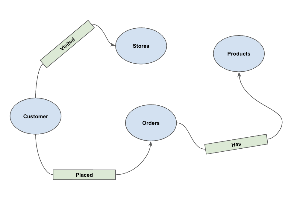
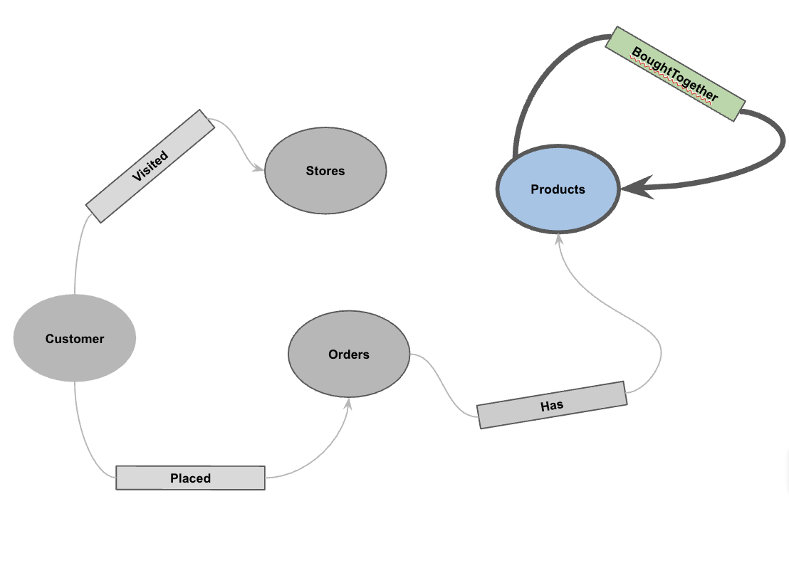
5. Create the Property Graph

With the data loaded, you can now define the property graph. This tells BigQuery which tables represent nodes (entities like Customers, Products) and which tables represent edges (relationships like "Visited", "Placed", "Has").

Run the following DDL statement:

CREATE OR REPLACE PROPERTY GRAPH cymbal_pets_demo.PetsOrderGraph
NODE TABLES (
  cymbal_pets_demo.customers KEY(customer_id) LABEL Customer,
  cymbal_pets_demo.products KEY(product_id) LABEL Products,
  cymbal_pets_demo.stores KEY(store_id) LABEL Stores,
  cymbal_pets_demo.orders KEY(order_id) LABEL Orders
)
EDGE TABLES (
  cymbal_pets_demo.orders as customer_to_store_edge
    KEY (order_id)
    SOURCE KEY (customer_id) references customers(customer_id)
    DESTINATION KEY (store_id) references stores(store_id)
    LABEL Visited
    PROPERTIES ALL COLUMNS,

  cymbal_pets_demo.order_items
    KEY (order_item_id)
    SOURCE KEY (order_id) references orders(order_id)
    DESTINATION KEY (product_id) references products(product_id)
    LABEL Has
    PROPERTIES ALL COLUMNS,

  cymbal_pets_demo.orders as customer_to_orders_edge
    KEY (order_id)
    SOURCE KEY (customer_id) references customers(customer_id)
    DESTINATION KEY (order_id) references orders(order_id)
    LABEL Placed
    PROPERTIES ALL COLUMNS,

  cymbal_pets_demo.co_related_products_for_angelica
    KEY (angelica_product_id)
    SOURCE KEY (angelica_product_id) references products(product_id)
    DESTINATION KEY (other_product_id) references products(product_id)
    LABEL BoughtTogether
    PROPERTIES ALL COLUMNS
);

This creates the graph PetsOrderGraph which allows us to perform graph traversals using the GRAPH_TABLE operator.

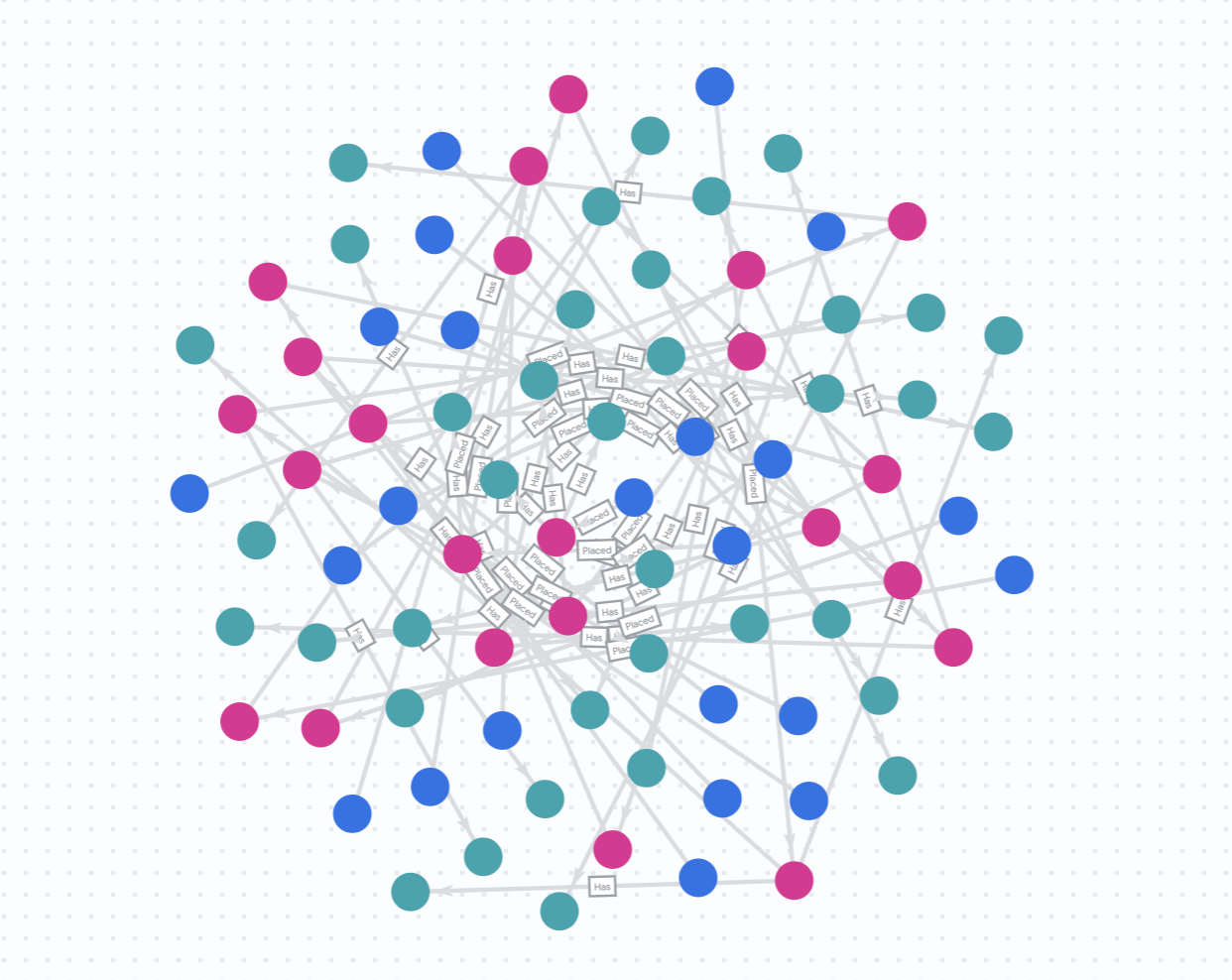
6. Visualize Purchase History of all customers

Open New Notebook in BigQuery Studio.

For the visualization and recommendation parts of this codelab, we will use a Google Colab notebook in BigQuery Studio. This allows us to easily visualize the graph results.

Paste the following into a code cell:

!pip install bigquery-magics==0.12.1

BigQuery Graph Notebook is implemented as an IPython Magics. By adding the %%bigquery magic command with the TO_JSON function, you can visualize the results as shown in the following sections.

Say that Cymbal Pets want to get a 360 degree visualization of all the customers and the purchases they did in a specific time window.

Run the following in a new cell:

%%bigquery --graph

GRAPH cymbal_pets_demo.PetsOrderGraph
  # finds the customer node and then finds all
  # the Orders nodes that are connected to that customer through the
  # Placed relationship
  MATCH (customer:Customer)-[placed:Placed]->(ordr:Orders)-[has:Has]->(product:Products)
  # filters the Orders nodes to only include those where the
  # order_date is within the last 3 months.
  WHERE ordr.order_date >= date('2024-11-27')
  # # This line finds all the Products nodes that are connected to the
  # # filtered Orders nodes through the Has relationship.
  MATCH p=(customer:Customer)-[placed:Placed]->(ordr:Orders)-[has:Has]->(product:Products)
  LIMIT 40
  RETURN 
    TO_JSON(p) as paths

BigQuery Graph allows you to match patterns across multiple tables without complex JOIN syntax.

You should see a visual representation of the graph result.

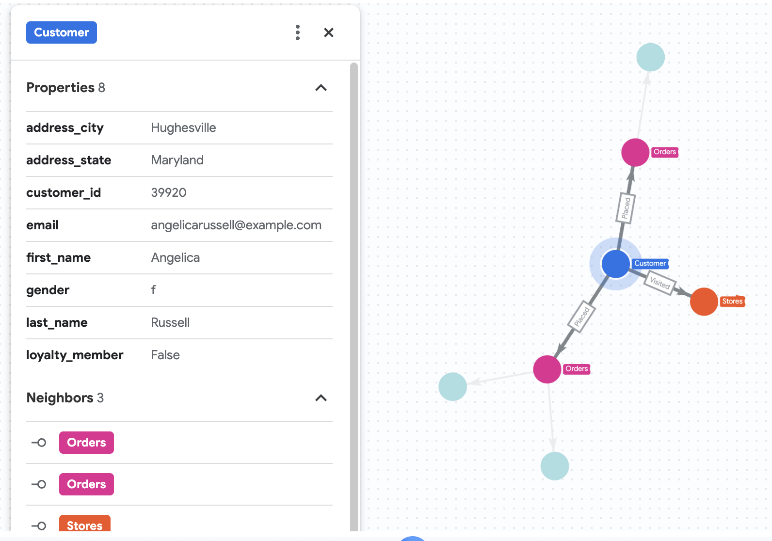
7. Visualize Purchase History of Angelica

Say that Cymbal Pets want to dive deep into a customer named Angelica Russell. They want to analyze the products that Angelica bought within the last 3 months, and the stores that the customer visited.

While this specific scenario could be achieved using a traditional relational join, we use BigQuery Graph here to demonstrate the fundamental graph concepts and syntax, which visualizes complex relationship analyses.

%%bigquery --graph

GRAPH cymbal_pets_demo.PetsOrderGraph
  # finds the customer node with the name "Angelica Russell" and then finds all
  # the Orders nodes that are connected to that customer through the
  # Placed relationship and all the Products nodes that are connected to the
  # filtered Orders nodes through the Has relationship.
   MATCH p=(customer:Customer {first_name: 'Angelica', last_name: 'Russell'})-[placed:Placed]->(ordr:Orders)-[has:Has]->(product:Products)
  # filters the Orders nodes to only include those where the
  # order_date is within the last 3 months.
  WHERE ordr.order_date >= date('2024-11-27')
  # finds the Stores nodes where Angelica placed order from
  MATCH p2=(customer)-[visited:Visited]->(store:Stores)
  RETURN
    TO_JSON(p) as path, TO_JSON(p2) as path2

8. Product Recommendation using vector search

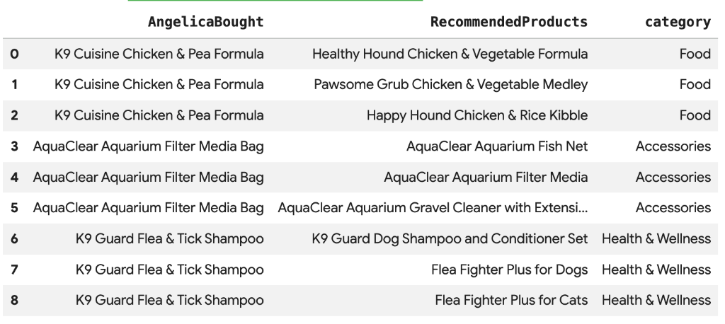
Cymbal Pets wants to recommend products to Angelica based on what she has bought recently. We can use vector search to find products with similar embeddings to her past purchases.

Run the following SQL script in a new Colab cell. This script:

1. Identifies products Angelica bought recently.
2. Uses VECTOR_SEARCH to find the top 4 similar products from the products table.

Note: This step assumes you have already run AI.GENERATE_EMBEDDINGS to create an embeddings column in the products table.

%%bigquery
DECLARE products_bought_by_angelica ARRAY<INT64>;

-- 1. Get IDs of products bought by Angelica
SET products_bought_by_angelica = (
  SELECT ARRAY_AGG(product_id) FROM
   GRAPH_TABLE(
    cymbal_pets_demo.PetsOrderGraph
      MATCH (c:Customer {first_name: 'Angelica', last_name: 'Russell'})-[placed:Placed]->(o:Orders)
      WHERE o.order_date >= date('2024-11-27')
      MATCH (o)-[has_edge:Has]->(p:Products)
      RETURN DISTINCT p.product_id as product_id
  ));

-- 2. Find similar products using vector search
SELECT 
  query.product_name as AngelicaBought, 
  base.product_name as RecommendedProducts, 
  base.category
FROM
  VECTOR_SEARCH(
    TABLE cymbal_pets_demo.products,
    'embedding',
    (SELECT * FROM cymbal_pets_demo.products
     WHERE product_id IN UNNEST(products_bought_by_angelica)),
    'embedding',
    top_k => 4)
WHERE query.product_name <> base.product_name;

You should see a list of recommended products that are semantically similar to what Angelica bought.

9. Recommendation using "Bought Together" and Jaccard Similarity

Another powerful recommendation technique is "Collaborative Filtering" — recommending products that are frequently bought together by other users.

We can find these products by traversing the graph from a customer to their purchased products, then to other customers who bought those products, and finally to the other products those customers bought.

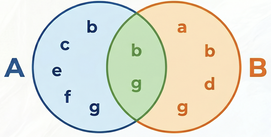
Overcoming Popularity Bias with Jaccard Similarity

While raw co-purchase counts are useful, they can be biased towards popular products. A very popular product might be bought with many things just by chance.

Jaccard Similarity takes recommendations one step further by normalizing the co-purchase count. It measures the similarity between two sets (in this case, the sets of orders containing each product).

The formula for Jaccard Similarity is:

Where:

• A intersect B is the number of orders containing both product A and product B (co-purchase count).
• A is the total number of orders containing product A.
• B is the total number of orders containing product B.

In the following example, set A = {b,c,e,f,g}, set B = {a,d,b,g}, their intersection A⋂B = {b,g}, their union A⋃B = {a,b,c,d,e,f,g}, hence the Jaccard similarity between A and B is 2 / 7 = 0.285714

Candidate Generation and Re-ranking

In real-world recommendation systems operating on massive datasets, it is often impractical to calculate complex similarity scores (like Jaccard) for all possible pairs of products. Instead, a common pattern is to use a two-stage approach:

1. Candidate Generation: Use a simple, fast metric (like raw co-purchase count) to filter the search space and find a manageable number of candidates (e.g., top 10).
2. Re-ranking: Apply a more precise, but computationally heavier, metric (like Jaccard Similarity) to rank that small set of candidates and select the final top recommendations.

In this codelab, we will follow this pattern:

• Stage 1: Run a query to find the top 10 co-purchased products for each product, based on raw co-purchase count, and store them in a table.
• Stage 2: Use a graph query to retrieve these candidates, rank them by Jaccard similarity, and return the top 3.

[!WARNING] Drawback: By filtering on raw count in Stage 1, we might lose "recall" of highly specific but low-frequency co-purchases. If a product is highly similar to another but both are rarely bought, it might not make it into the top 10 candidates and will be missed.

Run the following query to calculate both the raw co-purchase count and the Jaccard similarity, and store the top 10 candidates by raw count:

%%bigquery
CREATE OR REPLACE TABLE cymbal_pets_demo.co_related_products_for_angelica AS
-- Calculate the total number of orders for each product
WITH ProductOrderCounts AS (
    SELECT product_id, COUNT(DISTINCT order_id) as total_count
    FROM cymbal_pets_demo.order_items
    GROUP BY product_id
),
-- Calculate the intersection of each product pairs
CoPurchases AS (
    SELECT
        angelicaProduct.product_id AS angelica_product_id,
        otherProduct.product_id AS other_product_id,
        count(DISTINCT otherOrder.order_id) AS co_purchase_count
    FROM
        GRAPH_TABLE (cymbal_pets_demo.PetsOrderGraph
          MATCH (angelica:Customer {first_name: 'Angelica', last_name: 'Russell'})-[:Placed]->(o:Orders)-[:Has]->(angelicaProduct:Products)
          WHERE o.order_date >= date('2024-11-27')
          WITH angelica, angelicaProduct
          MATCH (otherCustomer:Customer)-[:Placed]->(otherOrder:Orders)-[:Has]->(angelicaProduct)
          WHERE otherCustomer <> angelica
          WITH angelicaProduct, otherOrder
          MATCH (otherOrder)-[:HAS]->(otherProduct:Products)
          WHERE angelicaProduct <> otherProduct
          RETURN angelicaProduct, otherProduct, otherOrder
        )
    GROUP BY
        angelicaProduct.product_id, otherProduct.product_id
)
SELECT * FROM (
    SELECT
        cp.angelica_product_id,
        cp.other_product_id,
        cp.co_purchase_count,
        -- The Jaccard calculation, which is the intersection of A and B divided by (A + B - intersection)
        SAFE_DIVIDE(cp.co_purchase_count, (poc1.total_count + poc2.total_count - cp.co_purchase_count)) AS jaccard_similarity,
        ROW_NUMBER() OVER (PARTITION BY cp.angelica_product_id ORDER BY cp.co_purchase_count DESC) AS rn
    FROM CoPurchases cp
    JOIN ProductOrderCounts poc1 ON cp.angelica_product_id = poc1.product_id
    JOIN ProductOrderCounts poc2 ON cp.other_product_id = poc2.product_id
)
WHERE rn <= 10;

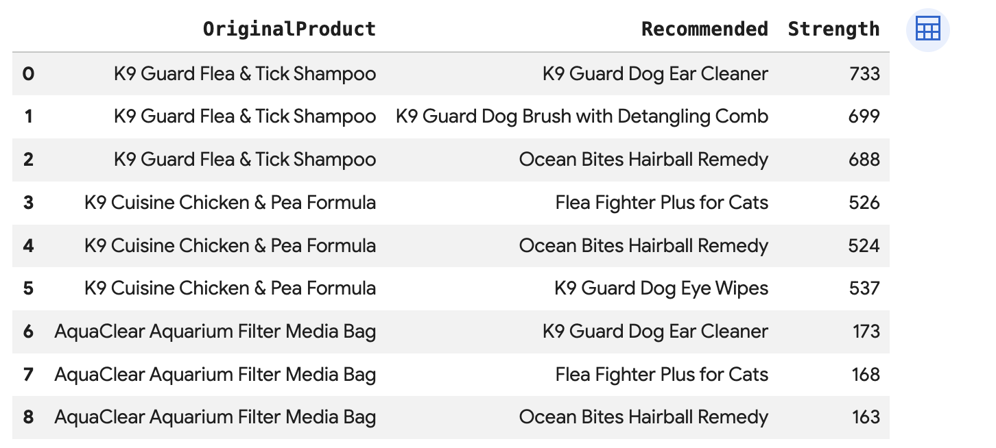
Run this query to recommend the top 3 products for each of Angelica's purchases, directly connected via the BoughtTogether edge, showing both the co-purchase count and Jaccard similarity:

%%bigquery
SELECT * FROM GRAPH_TABLE(
  cymbal_pets_demo.PetsOrderGraph
  MATCH (customer:Customer {first_name: 'Angelica', last_name: 'Russell'})-[placed:Placed]->(ordr:Orders)
  WHERE ordr.order_date >= date('2024-11-27')
  MATCH (ordr)-[has:Has]->(product:Products)
  MATCH (product)-[bought_together:BoughtTogether]->(recommended_product:Products)
  RETURN 
    product.product_name AS OriginalProduct,
    recommended_product.product_name AS Recommended,
    bought_together.co_purchase_count AS Strength,
    bought_together.jaccard_similarity AS JaccardSimilarity
)
-- Rank product recommendations by Jaccard Similarity
QUALIFY ROW_NUMBER() OVER (PARTITION BY OriginalProduct ORDER BY JaccardSimilarity DESC) <= 3
ORDER BY OriginalProduct;

This query traverses from Customer -> Order -> Product -> (BoughtTogether) -> Recommended Product, showing you recommendations based on collective purchase behavior and retrieves their similarity scores.

10. Clean up

To avoid ongoing charges to your Google Cloud account, delete the resources created during this codelab.

Delete the dataset and all tables:

DROP SCHEMA IF EXISTS cymbal_pets_demo CASCADE;

If you created a new project for this codelab, you can also delete the project:

gcloud projects delete $PROJECT_ID

11. Congratulations

Congratulations! You have successfully built a Customer 360 view and recommendation engine using BigQuery Graph.

What you've learned

• How to create a property graph in BigQuery.
• How to load data into graph nodes and edges.
• How to query graph patterns using GRAPH_TABLE and MATCH.
• How to combine graph queries with vector search for hybrid recommendations.

Next steps

• Explore BigQuery Graph documentation.
• Learn more about Vector Search in BigQuery.