Using Notebooks with Google Cloud Dataflow

1. Introduction

Google Cloud Dataflow

Last Updated: 2023-Jul-5

What is Dataflow?

Dataflow is a managed service for executing a wide variety of data processing patterns. The documentation on this site shows you how to deploy your batch and streaming data processing pipelines using Dataflow, including directions for using service features.

The Apache Beam SDK is an open source programming model that enables you to develop both batch and streaming pipelines. You create your pipelines with an Apache Beam program and then run them on the Dataflow service. The Apache Beam documentation provides in-depth conceptual information and reference material for the Apache Beam programming model, SDKs, and other runners.

Streaming data analytics with speed

Dataflow enables fast, simplified streaming data pipeline development with lower data latency.

Simplify operations and management

Allow teams to focus on programming instead of managing server clusters as Dataflow's serverless approach removes operational overhead from data engineering workloads.

Reduce total cost of ownership

Resource autoscaling paired with cost-optimized batch processing capabilities means Dataflow offers virtually limitless capacity to manage your seasonal and spiky workloads without overspending.

Key features

Automated resource management and dynamic work rebalancing

Dataflow automates provisioning and management of processing resources to minimize latency and maximize utilization so that you do not need to spin up instances or reserve them by hand. Work partitioning is also automated and optimized to dynamically rebalance lagging work. No need to chase down "hot keys" or preprocess your input data.

Horizontal autoscaling

Horizontal autoscaling of worker resources for optimum throughput results in better overall price-to-performance.

Flexible resource scheduling pricing for batch processing

For processing with flexibility in job scheduling time, such as overnight jobs, flexible resource scheduling (FlexRS) offers a lower price for batch processing. These flexible jobs are placed into a queue with a guarantee that they will be retrieved for execution within a six-hour window.

What you will run as part of this

Using the Apache Beam interactive runner with JupyterLab notebooks lets you iteratively develop pipelines, inspect your pipeline graph, and parse individual PCollections in a read-eval-print-loop (REPL) workflow. These Apache Beam notebooks are made available through Vertex AI Workbench, a managed service that hosts notebook virtual machines pre-installed with the latest data science and machine learning frameworks.

This codelab focuses on the functionality introduced by Apache Beam notebooks.

What you'll learn

• How to create a notebook instance
• Creating a basic pipeline
• Reading data from unbounded source
• Visualizing the data
• Launching a Dataflow Job from the notebook
• Saving a notebook

What you'll need

• A Google Cloud Platform project with Billing enabled.
• Google Cloud Dataflow and Google Cloud PubSub enabled.

2. Getting set up

1. In the Cloud Console, on the project selector page, select or create a Cloud project.

Note: If you don't plan to keep the resources that you create in this procedure, create a new project instead of selecting an existing project. After you finish these steps, you can delete the project, removing all resources associated with the project.

Go to project selector page

Ensure that you have the following APIs enabled:

• Dataflow API
• Cloud Pub/Sub API
• Compute Engine
• Notebooks API

You can verify this by checking on the API's & Services page.

Go to API's & Services Page

In this guide, we'll be reading data from a Pub/Sub subscription, therefore make sure that the Compute Engine default service account has the Editor role, or grant it the Pub/Sub Editor role.

3. Getting started with Apache Beam notebooks

Launching an Apache Beam notebooks instance

1. Launch Dataflow on the Console:

Go to Dataflow in the console

2. Select the Workbench page using the left-hand menu.
3. Make sure that you are on the User-managed notebooks tab.
4. In the toolbar, click New Notebook.
5. Select Apache Beam > Without GPUs.
6. On the New notebook page, select a subnetwork for the notebook VM and click Create.
7. Click Open JupyterLab when the link becomes active. Vertex AI Workbench creates a new Apache Beam notebook instance.

Note: After opening a user-managed notebooks instance, example notebooks are available in the Examples folder. The following are currently available:

• Word Count
• Streaming Word Count
• Streaming NYC Taxi Ride Data
• Dataflow Word Count
• Apache Beam SQL in notebooks
• Interactive Flink at Scale
• Use GPUs with Apache Beam
• Visualize Data

These notebooks include explanatory text and commented code blocks to help you understand Apache Beam concepts and API usage.

4. Creating the pipeline

Creating a notebook instance

Navigate to File > New > Notebook and select a kernel that is Apache Beam 2.47 or later.

Note: Apache Beam notebooks are built against the master branch of the Apache Beam SDK. This means that the latest version of the kernel shown in the notebooks UI might be ahead of the most recently released version of the SDK.

Start adding code to your notebook

• Copy and paste the code from each section within a new cell in your notebook
• Run the cell

Using the Apache Beam interactive runner with JupyterLab notebooks lets you iteratively develop pipelines, inspect your pipeline graph, and parse individual PCollections in a read-eval-print-loop (REPL) workflow.

Apache Beam is installed on your notebook instance, so include the interactive_runner and interactive_beam modules in your notebook.

import apache_beam as beam
from apache_beam.runners.interactive.interactive_runner import InteractiveRunner
import apache_beam.runners.interactive.interactive_beam as ib

If your notebook uses other Google services, add the following import statements:

from apache_beam.options import pipeline_options
from apache_beam.options.pipeline_options import GoogleCloudOptions
import google.auth

Setting interactivity options

The following sets the data capture duration to 60 seconds. If you want to iterate faster, set it to a lower duration, for example ‘10s'.

ib.options.recording_duration = '60s'

For additional interactive options, see the interactive_beam.options class.

Initialize the pipeline using an InteractiveRunner object.

# Setting up the Apache Beam pipeline options.
options = pipeline_options.PipelineOptions()

# Set the pipeline mode to stream the data from Pub/Sub.
options.view_as(pipeline_options.StandardOptions).streaming = True

# Sets the project to the default project in your current Google Cloud environment.
# The project will be used for creating a subscription to the Pub/Sub topic.
_, options.view_as(GoogleCloudOptions).project = google.auth.default()

# The Google Cloud PubSub topic for this example.
topic = "projects/pubsub-public-data/topics/shakespeare-kinglear"

p = beam.Pipeline(InteractiveRunner(), options=options)

Reading and visualizing the data

The following example shows an Apache Beam pipeline that creates a subscription to the given Pub/Sub topic and reads from the subscription.

words = p | "read" >> beam.io.ReadFromPubSub(topic=topic)

The pipeline counts the words by windows from the source. It creates fixed windowing with each window being 10 seconds in duration.

windowed_words = (words
   | "window" >> beam.WindowInto(beam.window.FixedWindows(10)))

After the data is windowed, the words are counted by window.

windowed_word_counts = (windowed_words
   | "count" >> beam.combiners.Count.PerElement())

Visualizing the data

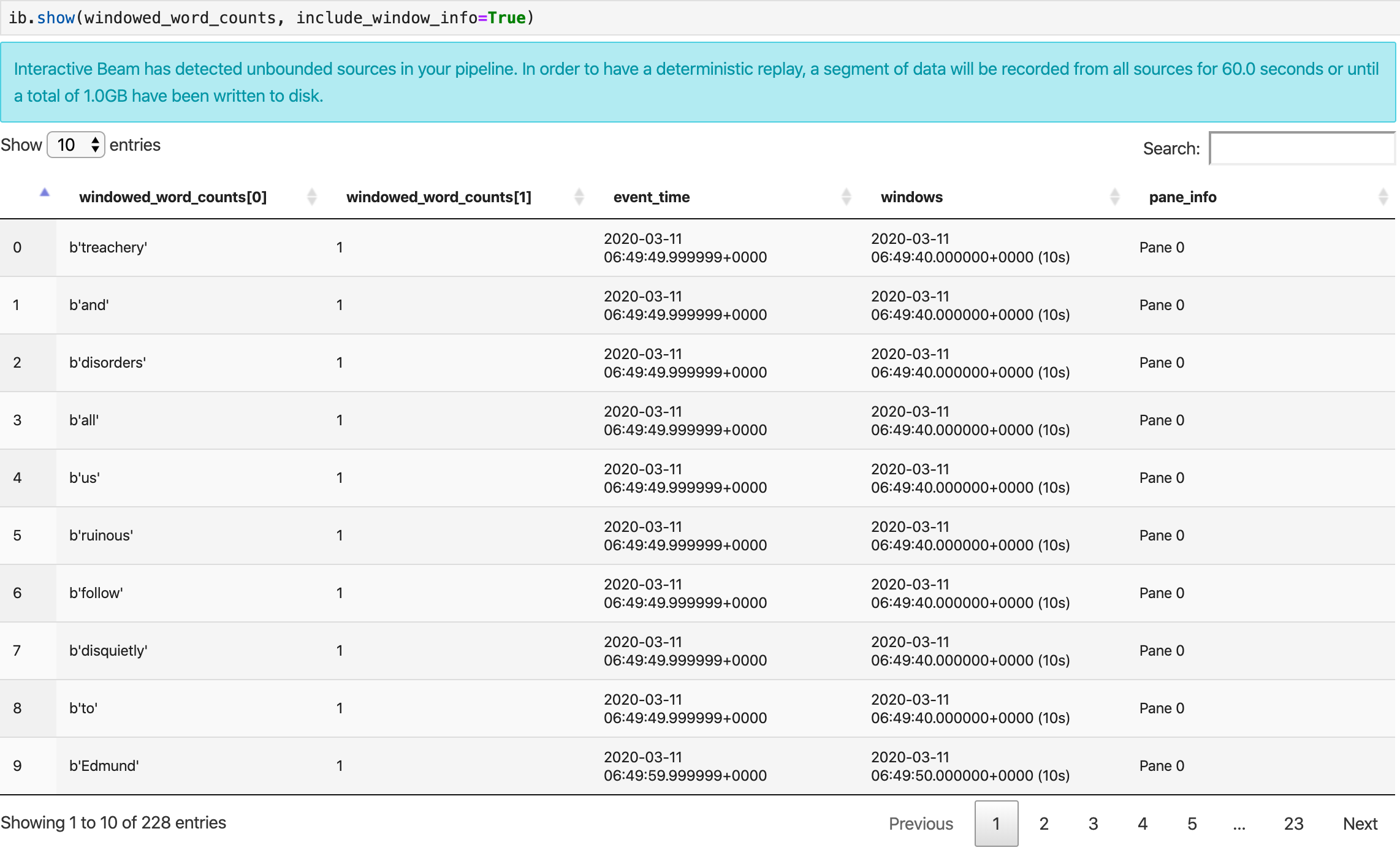
The show() method visualizes the resulting PCollection in the notebook.

ib.show(windowed_word_counts, include_window_info=True)

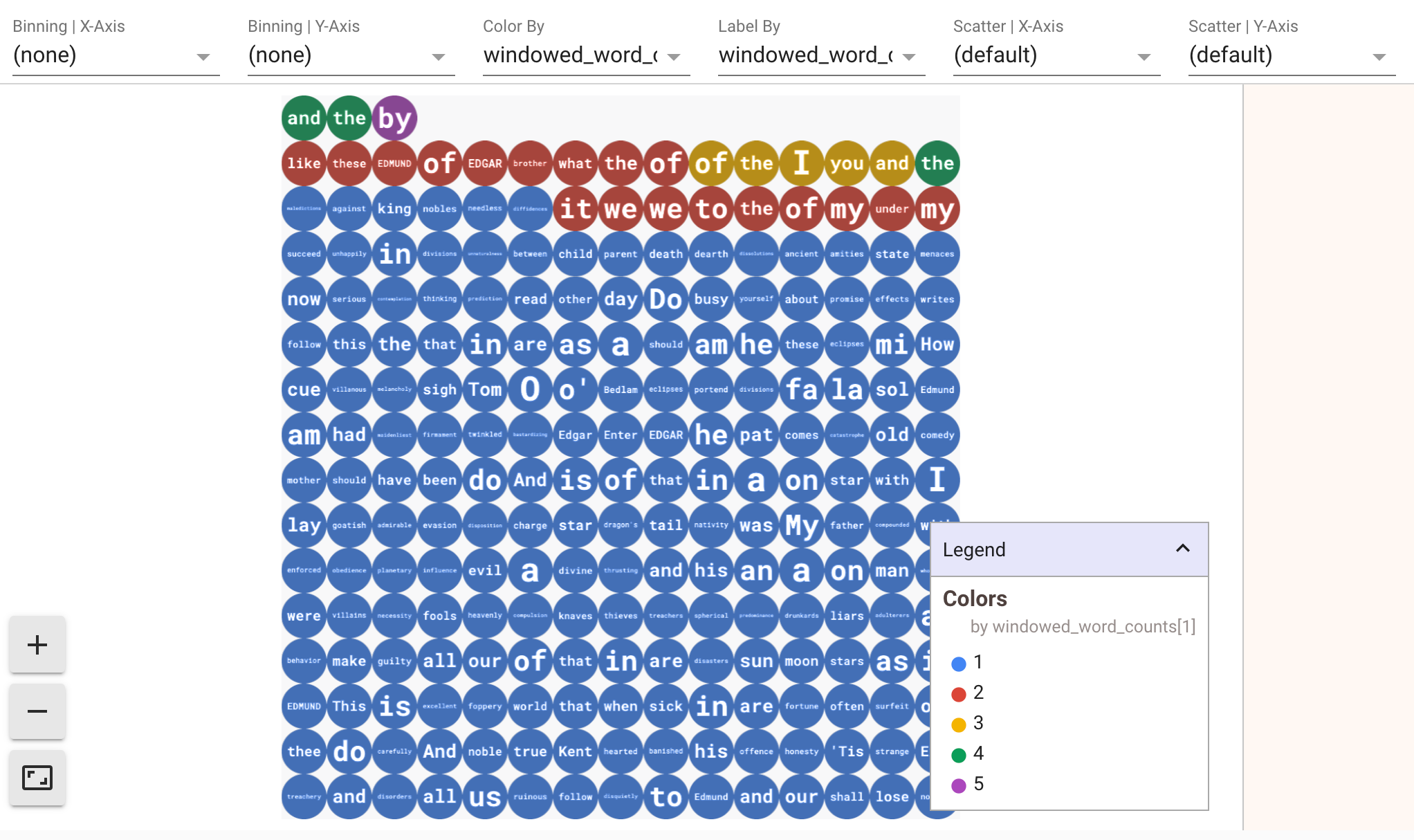
To display visualizations of your data, pass visualize_data=True into the show() method. Add a new cell:

ib.show(windowed_word_counts, include_window_info=True, visualize_data=True)

You can apply multiple filters to your visualizations. The following visualization allows you to filter by label and axis:

Note: To ensure replayability while prototyping streaming pipelines, the show() method calls reuse the captured data by default. By setting interactive_beam.options.enable_capture_replay = False, you can change this behavior and have the show() method always fetch new data. Also, if you add a second unbounded source to your notebook, the data from the previous unbounded source is discarded.

5. Using a Pandas Dataframe

Another useful visualization in Apache Beam notebooks is a Pandas DataFrame. The following example first converts the words to lowercase and then computes the frequency of each word.

windowed_lower_word_counts = (windowed_words
   | "to lower case" >> beam.Map(lambda word: word.lower())
   | "count lowered" >> beam.combiners.Count.PerElement())

The collect() method provides the output in a Pandas DataFrame.

ib.collect(windowed_lower_word_counts, include_window_info=True)

Note: Editing and re-executing a cell is a common practice in notebook development. When you edit and re-execute a cell in a Apache Beam notebook, the cell does not undo the intended action of the code in the original cell. For example, if a cell adds a PTransform to a pipeline, re-executing that cell would add an additional PTransform to the pipeline. If you want to clear the state, restart the kernel and rerun the cells.

6. (Optional) Launching Dataflow jobs from your notebook

1. To run jobs on Dataflow, you need additional permissions. Make sure the Compute Engine default service account has the Editor role, or grant it the following IAM roles:

• Dataflow Admin
• Dataflow Worker
• Storage Admin, and
• Service Account User (roles/iam.serviceAccountUser)

See more about roles in the documentation.

2. (Optional) Before using your notebook to run Dataflow jobs, restart the kernel, rerun all cells, and verify the output.
3. Remove the following import statements:

from apache_beam.runners.interactive.interactive_runner import InteractiveRunner
import apache_beam.runners.interactive.interactive_beam as ib

4. Add the following import statement:

from apache_beam.runners import DataflowRunner

5. Remove the following recording duration option:

ib.options.recording_duration = '60s'

6. Add the following to your pipeline options. You will need to adjust the Cloud Storage location to point to a bucket you already own, or you can create a new bucket for this purpose. You can also change the region value from us-central1.

# Set the Google Cloud region to run Dataflow.
options.view_as(GoogleCloudOptions).region = 'us-central1'

# Choose a Cloud Storage location.
dataflow_gcs_location = 'gs://<change me>/dataflow'

# Choose a location for your output files
output_gcs_location = '%s/results/' % dataflow_gcs_location


# Set the staging location. This location is used to stage the
# Dataflow pipeline and SDK binary.
options.view_as(GoogleCloudOptions).staging_location = '%s/staging' % dataflow_gcs_location

# Set the temporary location. This location is used to store temporary files
# or intermediate results before outputting to the sink.
options.view_as(GoogleCloudOptions).temp_location = '%s/temp' % dataflow_gcs_location

7. In the constructor of beam.Pipeline(), replace InteractiveRunner with DataflowRunner. p is the pipeline object from creating your pipeline.

p = beam.Pipeline(DataflowRunner(), options=options)

8. Remove the interactive calls from your code. For example, remove show(), collect(), head(), show_graph(), and watch() from your code.
9. To be able to see any results you will need to add a sink. In the previous section we were visualizing results in the notebook, but this time, we're running the job outside of this notebook - in Dataflow. Therefore, we need an external location for our results. In this example, we'll write the results to text files in GCS (Google Cloud Storage). Since this is a streaming pipeline, with data windowing, we'll want to create one text file per window. To achieve this, add the following steps to your pipeline:

result = (windowed_lower_word_counts
    | "decode words and format" >> beam.Map(lambda x: f"{x[0].decode('utf-8')}: {x[1]}")
    | "write events to file" >> beam.io.fileio.WriteToFiles(path=output_gcs_location, shards=1, max_writers_per_bundle=0))

10. Add p.run() at the end of your pipeline code.
11. Now review your notebook code to confirm you've incorporated all of the changes. It should look similar to this:

import apache_beam as beam
from apache_beam.options import pipeline_options
from apache_beam.options.pipeline_options import GoogleCloudOptions
import google.auth
from apache_beam.runners import DataflowRunner

# Setting up the Apache Beam pipeline options.
options = pipeline_options.PipelineOptions()

# Set the pipeline mode to stream the data from Pub/Sub.
options.view_as(pipeline_options.StandardOptions).streaming = True

# Sets the project to the default project in your current Google Cloud environment.
# The project will be used for creating a subscription to the Pub/Sub topic.
_, options.view_as(GoogleCloudOptions).project = google.auth.default()

# Set the Google Cloud region to run Dataflow.
options.view_as(GoogleCloudOptions).region = 'us-central1'

# Choose a Cloud Storage location.
dataflow_gcs_location = 'gs://<change me>/dataflow'

# Choose a location for your output files
output_gcs_location = '%s/results/' % dataflow_gcs_location


# Set the staging location. This location is used to stage the
# Dataflow pipeline and SDK binary.
options.view_as(GoogleCloudOptions).staging_location = '%s/staging' % dataflow_gcs_location

# Set the temporary location. This location is used to store temporary files
# or intermediate results before outputting to the sink.
options.view_as(GoogleCloudOptions).temp_location = '%s/temp' % dataflow_gcs_location



# The Google Cloud PubSub topic for this example.
topic = "projects/pubsub-public-data/topics/shakespeare-kinglear"

p = beam.Pipeline(DataflowRunner(), options=options)
words = p | "read" >> beam.io.ReadFromPubSub(topic=topic)
windowed_words = (words
   | "window" >> beam.WindowInto(beam.window.FixedWindows(10)))

windowed_words_counts = (windowed_words
   | "count" >> beam.combiners.Count.PerElement())

windowed_lower_word_counts = (windowed_words
   | "to lower case" >> beam.Map(lambda word: word.lower())
   | "count lowered" >> beam.combiners.Count.PerElement())

result = (windowed_lower_word_counts
    | "decode words and format" >> beam.Map(lambda x: f"{x[0].decode('utf-8')}: {x[1]}")
    | "write events to file" >> beam.io.fileio.WriteToFiles(path=output_gcs_location, shards=1, max_writers_per_bundle=0))

p.run()

12. Run the cells.
13. You should see a similar output to the following:

<DataflowPipelineResult <Job
 clientRequestId: '20230623100011457336-8998'
 createTime: '2023-06-23T10:00:33.447347Z'
 currentStateTime: '1970-01-01T00:00:00Z'
 id: '2023-06-23_03_00_33-11346237320103246437'
 location: 'us-central1'
 name: 'beamapp-root-0623075553-503897-boh4u4wb'
 projectId: 'your-project-id'
 stageStates: []
 startTime: '2023-06-23T10:00:33.447347Z'
 steps: []
 tempFiles: []
 type: TypeValueValuesEnum(JOB_TYPE_STREAMING, 2)> at 0x7fc7e4084d60>

14. To validate if the job is running, go to the Jobs page for Dataflow. You should see a new job on the list. The job will take around ~5-10 minutes to start processing the data.
15. Once data is processing, head to Cloud Storage and navigate to the directory where Dataflow is storing the results (your defined output_gcs_location). You should see a list of text files, with one file per window.
16. Download the file and inspect the content. It should contain the list of words paired with their count. Alternatively, use the command line interface to inspect the files. You can do it by running the following in a new cell in your notebook:

! gsutils cat gs://<your-bucket-here>/results/<file-name>

17. You will see a similar output to this:

Safer: 1

trust: 1

mercy: 1

harms: 1

far: 2

fear: 1

than: 1

take: 1

me: 1

goneril: 1

still: 1

away: 1

let: 1

too: 2

the: 1

18. That's it! Don't forget to clean up and stop the job you've created (see final step of this codelab).

For an example on how to perform this conversion on an interactive notebook, see the Dataflow Word Count notebook in your notebook instance.

Alternatively, you can export your notebook as an executable script, modify the generated .py file using the previous steps, and then deploy your pipeline to the Dataflow service.

7. Saving your notebook

Notebooks you create are saved locally in your running notebook instance. If you reset or shut down the notebook instance during development, those new notebooks are persisted as long as they are created under the /home/jupyter directory. However, if a notebook instance is deleted, those notebooks are also deleted.

To keep your notebooks for future use, download them locally to your workstation, save them to GitHub, or export them to a different file format.

8. Cleaning up

After you've finished using your Apache Beam notebook instance, clean up the resources you created on Google Cloud by shutting down the notebook instance and stopping the streaming job, if you've run one.

Alternatively, if you've created a project for the sole purpose of this codelab, you may also shut down the project entirely.