Fraud Detection with BigQuery Graph

1. Introduction

Fraudulent activity often involves hidden networks of connected entities—for example, multiple accounts sharing the same email address, phone number, or physical address. Traditional relational databases can struggle to query these complex, multi-hop relationships efficiently.

BigQuery Graph allows you to analyze these networks at scale using graph databases. You can define a property graph on top of your existing BigQuery tables and use Graph Query Language (GQL) to find patterns in your data.

A common application of graph networks for fraud detection is stopping orders that have a delivery address associated with a fraud network or stopping payments belonging to .

In this codelab, you will build a fraud detection solution using BigQuery Graph. You will load data from Cloud Storage, create a property graph, and use graph queries to identify suspicious connections.

What you'll learn

• How to create a BigQuery dataset and load data.
• How to define a property graph using DDL.
• How to query the graph using GQL.
• How to use graph analytics to detect fraud.

What you'll need

• A Google Cloud project with billing enabled.
• A BigQuery notebook environment (BigQuery Studio or Colab Enterprise).

Cost

This lab uses Google Cloud resources that are billable. The estimated cost is under $5, assuming you delete the resources after completion.

2. Before you begin

Select or create a Google Cloud project

1. In the Google Cloud Console, on the project selector page, select or create a Google Cloud project.
2. Make sure that billing is enabled for your Google Cloud project. Learn how to check if billing is enabled.

Choose your environment

You will need a notebook environment to run this lab. You can use BigQuery Studio or Colab Enterprise.

1. Navigate to the BigQuery page in the Google Cloud Console.
2. You will use the python notebook to run the graph queries.

Start Cloud Shell

1. Click Activate Cloud Shell at the top of the Google Cloud console.
2. Verify authentication:

gcloud auth list

3. Confirm your project:

gcloud config get project

4. Set it if needed:

export PROJECT_ID=<YOUR_PROJECT_ID>
gcloud config set project $PROJECT_ID

Enable APIs

Run this command to enable the required BigQuery API:

gcloud services enable bigquery.googleapis.com

3. Load Data

In this step, you will create a BigQuery dataset and load the sample data from Cloud Storage.

The sample data consists of several CSV files representing a simulated retail environment:

• customers.csv: Customer account information.
• emails.csv: Email addresses.
• phones.csv: Phone numbers.
• addresses.csv: Physical addresses.
• customer_emails.csv, customer_phones.csv, customer_addresses.csv: Linking tables.
• orders.csv: Order history, including fraud flags.

Create the Dataset

Create a dataset named fraud_demo to hold the tables.

1. For this codelab, we will execute SQL commands. You can run these commands in the BigQuery Studio > SQL Editor, or use the bq query command in Cloud Shell. We will assume you are using the BigQuery SQL Editor for a better experience with multi-line create statements.

CREATE SCHEMA IF NOT EXISTS `fraud_demo` OPTIONS(location="US");

Load Tables

Run the following SQL statements to load data from Cloud Storage into your dataset.

LOAD DATA OVERWRITE `fraud_demo.customers`
FROM FILES (
  format = 'CSV',
  uris = ['gs://sample-data-and-media/fraud-demo-data/customers.csv'],
  skip_leading_rows = 1
);

LOAD DATA OVERWRITE `fraud_demo.emails`
FROM FILES (
  format = 'CSV',
  uris = ['gs://sample-data-and-media/fraud-demo-data/emails.csv'],
  skip_leading_rows = 1
);

LOAD DATA OVERWRITE `fraud_demo.phones`
FROM FILES (
  format = 'CSV',
  uris = ['gs://sample-data-and-media/fraud-demo-data/phones.csv'],
  skip_leading_rows = 1
);

LOAD DATA OVERWRITE `fraud_demo.addresses`
FROM FILES (
  format = 'CSV',
  uris = ['gs://sample-data-and-media/fraud-demo-data/addresses.csv'],
  skip_leading_rows = 1
);

LOAD DATA OVERWRITE `fraud_demo.customer_emails`
FROM FILES (
  format = 'CSV',
  uris = ['gs://sample-data-and-media/fraud-demo-data/customer_emails.csv'],
  skip_leading_rows = 1
);

LOAD DATA OVERWRITE `fraud_demo.customer_phones`
FROM FILES (
  format = 'CSV',
  uris = ['gs://sample-data-and-media/fraud-demo-data/customer_phones.csv'],
  skip_leading_rows = 1
);

LOAD DATA OVERWRITE `fraud_demo.customer_addresses`
FROM FILES (
  format = 'CSV',
  uris = ['gs://sample-data-and-media/fraud-demo-data/customer_addresses.csv'],
  skip_leading_rows = 1
);

LOAD DATA OVERWRITE `fraud_demo.orders`
FROM FILES (
  format = 'CSV',
  uris = ['gs://sample-data-and-media/fraud-demo-data/orders.csv'],
  skip_leading_rows = 1
);

4. Create the Property Graph

Now that the data is loaded, you can define the property graph. A property graph consists of nodes (entities) and edges (relationships).

In this lab, the nodes are:

• Customer: Represents the account holder.
• Phone: Represents a phone number.
• Email: Represents an email address.
• Address: Represents a physical address.

The edges are:

• OwnsPhone: Connects a Customer to a Phone.
• OwnsEmail: Connects a Customer to an Email.
• LinkedToAddress: Connects a Customer to an Address.

Create the Graph

Run the following DDL statement to create the graph named FraudDemo in your fraud_demo dataset.

CREATE OR REPLACE PROPERTY GRAPH fraud_demo.FraudDemo
  NODE TABLES(
    fraud_demo.customers
      KEY(account_id)
      LABEL Customer PROPERTIES(
        account_id,
        name),

    fraud_demo.emails
      KEY(email)
      LABEL Email PROPERTIES(
        email,
        email_type),

    fraud_demo.phones
      KEY(phone_number)
      LABEL Phone PROPERTIES(
        phone_number,
        phone_type),

    fraud_demo.addresses
      KEY(address)
      LABEL Address PROPERTIES(
        address,
        address_type)
  )
  EDGE TABLES(
    fraud_demo.customer_emails
      KEY(account_id, email)
      SOURCE KEY(account_id) REFERENCES customers(account_id)
      DESTINATION KEY(email) REFERENCES emails(email)
      LABEL OwnsEmail PROPERTIES(
        account_id,
        email,
        last_updated_ts),

    fraud_demo.customer_phones
      KEY(account_id, phone_number)
      SOURCE KEY(account_id) REFERENCES customers(account_id)
      DESTINATION KEY(phone_number) REFERENCES phones(phone_number)
      LABEL OwnsPhone PROPERTIES(
        account_id,
        phone_number,
        last_updated_ts),

    fraud_demo.customer_addresses
      KEY(account_id, address)
      SOURCE KEY(account_id) REFERENCES customers(account_id)
      DESTINATION KEY(address) REFERENCES addresses(address)
      LABEL LinkedToAddress PROPERTIES(
        account_id,
        address,
        last_updated_ts)
  );

5. Analyze Networks (2-Hop)

Open New Notebook in BigQuery Studio.

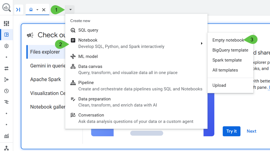
For the visualization and recommendation parts of this codelab, we will use a Google Colab notebook in BigQuery Studio. This allows us to easily visualize the graph results.

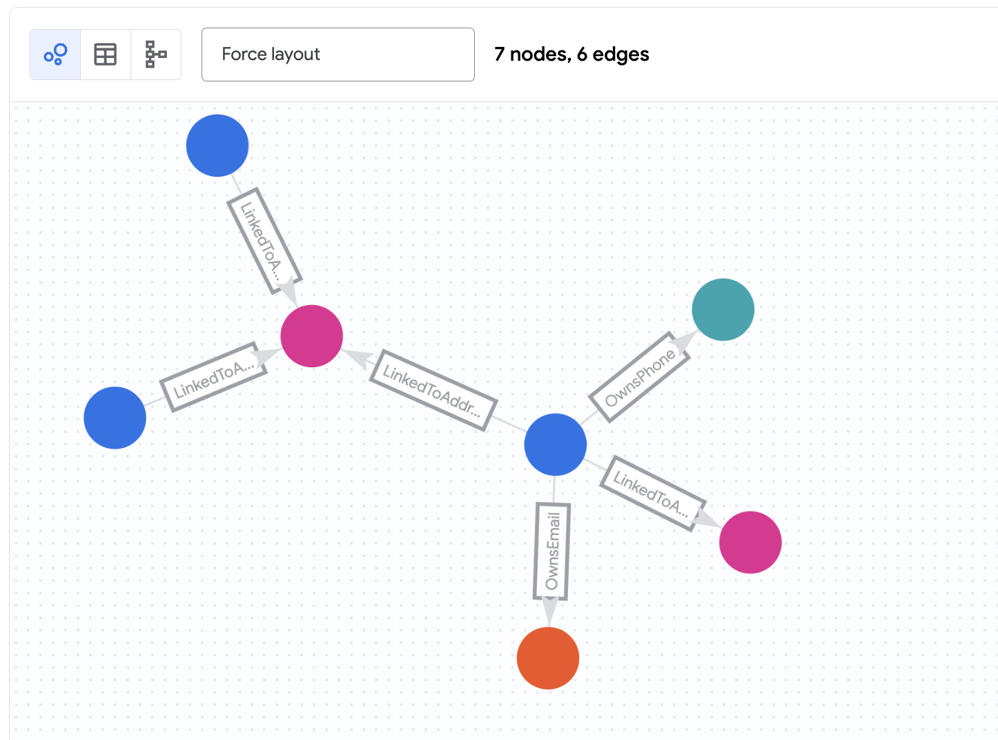
BigQuery Graph Notebook is implemented as an IPython Magics. By adding the %%bigquery magic command with the TO_JSON function, you can visualize the results as shown in the following sections. In this step, you will run a graph query to find simple connections between accounts. This is a "2-hop" query because it travels 2 hops out from a starting node to find related nodes (e.g., Customer -> Email -> Customer).

We will start by investigating the account belonging to Nicole Wade. We want to find any accounts related to her via 2 hops.

Run the 2-Hop Query

Run the following query in your notebook.

%%bigquery --graph
GRAPH fraud_demo.FraudDemo
MATCH 
 p=(a:Customer) 
  ( -[e:OwnsEmail|OwnsPhone|LinkedToAddress WHERE e.last_updated_ts < '2025-07-30']- (n) ){2}
WHERE a.account_id IN ("d2f1f992-d116-41b3-955b-6c76a3352657")
  -- Verify the final node in the hop array is a Customer
  AND 'Customer' IN UNNEST(LABELS(n[OFFSET(1)]))

RETURN TO_JSON(p) AS paths

Understand the Results

This query:

1. Starts at the Customer node with account_id "d2f1f992-d116-41b3-955b-6c76a3352657" (Nicole Wade).
2. Follows any of the edges OwnsEmail, OwnsPhone, or LinkedToAddress to a connecting node (Phone, Email, or Address).
3. Follows edges back from that connecting node to other Customer nodes.
4. Filters edges based on a timestamp (last_updated_ts) to see the state of the network at a specific time.

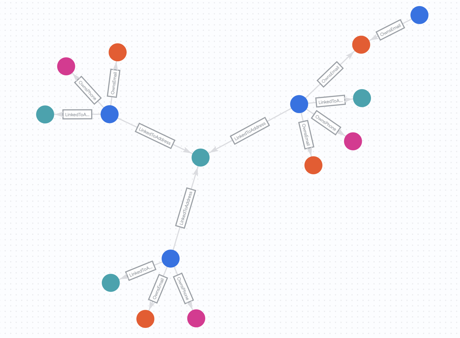
You should see that Zachary Cordova and Brenda Brown are connected to Nicole via the same address.

6. Analyze Networks (4-Hop)

In this step, you will extend the query to find more complex relationships. We will look for 4-hop connections. This allows us to find accounts that are connected through several intermediate entities (e.g., Customer A -> Email -> Customer B -> Phone -> Customer C).

We will also observe how this network changes over time.

The "Before" State

First, let's look at the network as it existed on July 30, 2025.

Run the following query:

%%bigquery --graph
%%bigquery --graph

MATCH p= ANY SHORTEST (a:Customer) 
  ( -[e:OwnsEmail|OwnsPhone|LinkedToAddress WHERE e.last_updated_ts < '2025-07-30']- (n) ){3, 5}(reachable_a:Customer)
WHERE a.account_id IN ("d2f1f992-d116-41b3-955b-6c76a3352657")
  -- Ensure the final node in the dynamic chain is actually a Customer
  AND 'Customer' IN UNNEST(LABELS(n[OFFSET(ARRAY_LENGTH(n) - 1)]))
GRAPH fraud_demo.FraudDemo
RETURN 
  TO_JSON(p) AS paths,                   -- Array of all traversed edges
  ARRAY_LENGTH(e) AS hop_count

The "After" State

Now, let's see how the network looks 2 weeks later. We will run the same query but without the date restrictions.

Run the following query:

%%bigquery --graph
GRAPH fraud_demo.FraudDemo
MATCH p= ANY SHORTEST (a:Customer) 
  ( -[e:OwnsEmail|OwnsPhone|LinkedToAddress]- (n) ){3, 5}(reachable_a:Customer)
WHERE a.account_id IN ("d2f1f992-d116-41b3-955b-6c76a3352657")
  -- Ensure the final node in the dynamic chain is actually a Customer
  AND 'Customer' IN UNNEST(LABELS(n[OFFSET(ARRAY_LENGTH(n) - 1)]))

RETURN 
  TO_JSON(p) AS paths,                   -- Array of all traversed edges
  ARRAY_LENGTH(e) AS hop_count

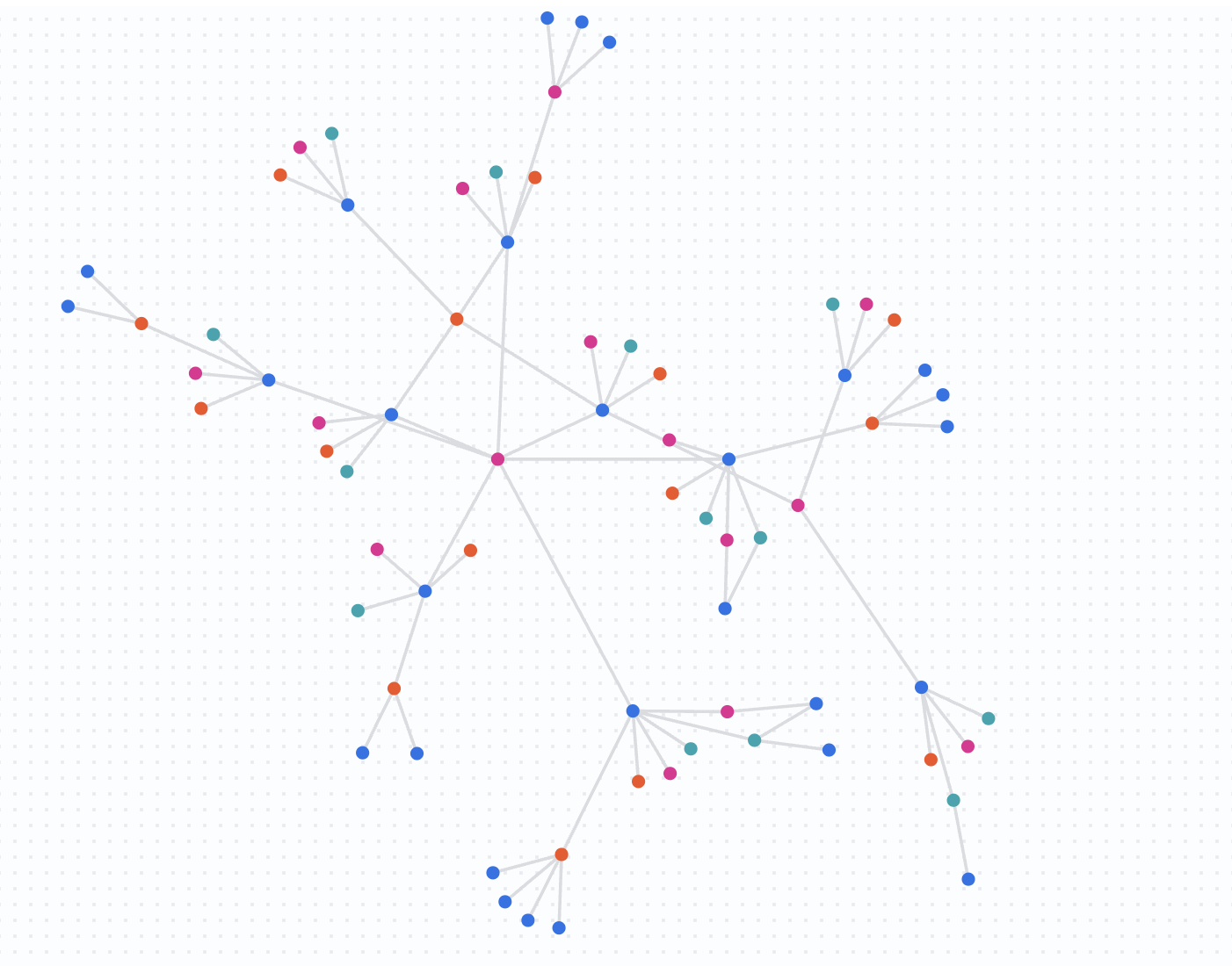
Understand the Results

By removing the date filters, you are query against the full dataset. You will notice that the network has grown significantly. Nicole Wade is now part of a much larger, highly connected group. This rapid expansion of a connected network is a strong indicator of potentially fraudulent activity, such as a fraud ring sharing resources over time.

7. Generate Fraud Report

In this step, you will combine graph analytics with traditional business data (orders) to generate a comprehensive fraud report. You will identify accounts at risk and potential fraudulent orders.

This query is more complex. It uses GRAPH_TABLE to run the graph query inside standard SQL and calculates the change in network size (diff) between the "before" and "after" states we observed in the previous step.

Run the Fraud Report Query

Run the following query in your notebook.

%%bigquery --graph
WITH num_orders AS (
  SELECT account_id, COUNT(1) AS num_order
  FROM fraud_demo.orders
  WHERE order_time > '2025-07-30'
  GROUP BY account_id
),

orders AS (
  SELECT account_id, order_id, fraud, order_total
  FROM fraud_demo.orders
  WHERE order_time > '2025-07-30'
),

-- Use Quantified Path Patterns to find connections up to 4 hops away
latest_connect AS (
  SELECT 
    account_id, 
    ARRAY_LENGTH(ARRAY_AGG(DISTINCT connected_id)) AS size
  FROM GRAPH_TABLE(
    fraud_demo.FraudDemo
    MATCH (a:Customer)-[:OwnsEmail|OwnsPhone|LinkedToAddress]-{4}(connected:Customer)
    RETURN a.account_id AS account_id, connected.account_id AS connected_id
  )
  GROUP BY account_id
),

prev_connect AS (
  SELECT 
    account_id, 
    ARRAY_LENGTH(ARRAY_AGG(DISTINCT connected_id)) AS size
  FROM GRAPH_TABLE(
    fraud_demo.FraudDemo
    -- Apply the timestamp filter to EVERY edge in the 4-hop chain
    MATCH (a:Customer)
          (-[e:OwnsEmail|OwnsPhone|LinkedToAddress WHERE e.last_updated_ts < '2025-07-30']-(n)){4}
    WHERE 'Customer' IN UNNEST(LABELS(n[OFFSET(3)]))
    RETURN a.account_id AS account_id, n[OFFSET(3)].account_id AS connected_id
  )
  GROUP BY account_id
),

edge_changes AS (
  SELECT account_id, MAX(last_updated_ts) AS max_last_updated_ts
  FROM fraud_demo.customer_addresses
  GROUP BY account_id
)

SELECT
    la.account_id,
    o.order_id,
    la.size AS latest_size,
    COALESCE(pa.size, 0) AS previous_size,
    la.size - COALESCE(pa.size, 0) AS diff,
    nos.num_order,
    o.fraud AS reported_as_fraud,
    o.order_total,

    CASE
      WHEN (la.size - COALESCE(pa.size, 0)) > 10 AND nos.num_order IS NULL THEN "CUSTOMER AT RISK"
      WHEN (la.size - COALESCE(pa.size, 0)) > 10 AND nos.num_order IS NOT NULL AND o.fraud THEN "CONFIRMED FRAUD ORDER"
      WHEN (la.size - COALESCE(pa.size, 0)) > 10 AND nos.num_order IS NOT NULL AND NOT o.fraud THEN "POTENTIAL FRAUD ORDER"
      ELSE ""
    END AS notes
FROM latest_connect la
LEFT JOIN prev_connect pa ON la.account_id = pa.account_id
LEFT JOIN num_orders nos ON la.account_id = nos.account_id
LEFT JOIN orders o ON la.account_id = o.account_id
INNER JOIN edge_changes ec ON la.account_id = ec.account_id
WHERE nos.num_order > 1 OR (la.size - COALESCE(pa.size, 0)) > 10
ORDER BY diff DESC

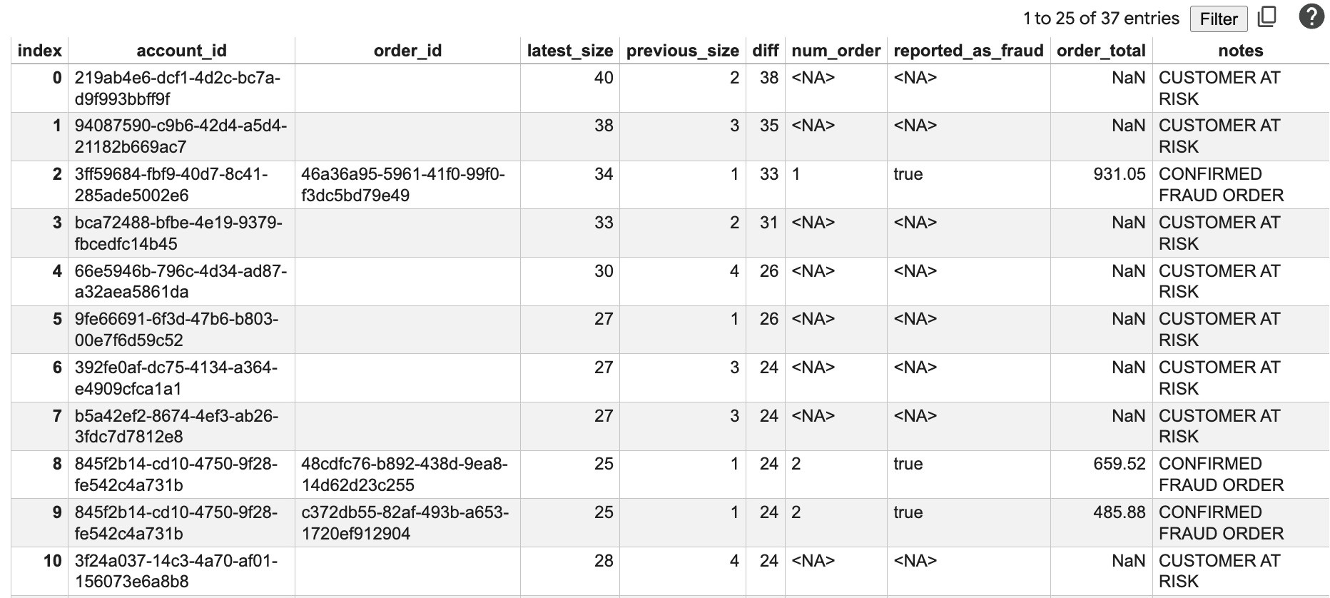
Understand the Results

This report shows:

• account_id: The ID of the account being analyzed.
• order_id: A recent order ID.
• latest_size: The size of the connected network today.
• previous_size: The size of the network 2 weeks ago.
• diff: The growth in the network size.
• num_order: The number of recent orders.
• reported_as_fraud: Whether the order has been flagged as fraud.
• order_total: The total amount of the order.
• notes: A calculated risk status based on network growth and order history.

You will see accounts with large diff values and high order totals, which are prime candidates for further investigation. The "CUSTOMER AT RISK" and "POTENTIAL FRAUD ORDER" notes help prioritize these accounts.

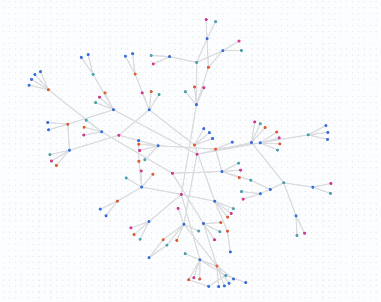
8. Detection at Scale

In this final analysis step, you will visualize the network at a larger scale. Instead of starting with a single account, you will query for connections among a set of suspicious accounts.

This helps you see if multiple independent investigations are actually part of the same larger fraud ring.

Run the Scaled Query

Run the following query in your notebook.

%%bigquery --graph
GRAPH fraud_demo.FraudDemo
MATCH
p= ANY SHORTEST (a:Customer) 
  ( -[e:OwnsEmail|OwnsPhone|LinkedToAddress]- (n) ){3, 5}
(reachable_a:Customer)
-- these IDs are from the previous results
WHERE a.account_id in (   "845f2b14-cd10-4750-9f28-fe542c4a731b"
  , "3ff59684-fbf9-40d7-8c41-285ade5002e6"
  , "8887c17b-e6fb-4b3b-8c62-cb721aafd028"
  , "03e777e5-6fb4-445d-b48c-cf42b7620874"
  , "81629832-eb1d-4a0e-86da-81a198604898"
  , "845f2b14-cd10-4750-9f28-fe542c4a731b",
   "89e9a8fe-ffc4-44eb-8693-a711a3534849"
 )
 LIMIT 400
RETURN TO_JSON(p) as paths

Understand the Results

This query returns a complex graph showing how the specified suspicious accounts overlap and share resources. You are now looking at fraud detection at scale, identifying clusters of activity that might warrant a coordinated response.

9. Clean Up

To avoid incurring charges to your Google Cloud account for the resources used in this codelab, you should delete the dataset and the property graph.

Run the following SQL statements to clean up your environment.

DROP PROPERTY GRAPH IF EXISTS fraud_demo.FraudDemo;
DROP SCHEMA IF EXISTS fraud_demo CASCADE;

10. Congratulations

Congratulations! You have successfully built a fraud detection solution using BigQuery Graph.

You have learned how to:

• Load data from Cloud Storage into BigQuery.
• Define a property graph using DDL.
• Query the graph using GQL to find simple and complex relationships.
• Combine graph analytics with business data to identify risk.
• Visualize networks at scale.

More Resources

• BigQuery Graph Documentation