Your first Keras model, with transfer learning

1. Overview

In this lab, you will learn how to build a Keras classifier. Instead of trying to figure out the perfect combination of neural network layers to recognize flowers, we will first use a technique called transfer learning to adapt a powerful pre-trained model to our dataset.

This lab includes the necessary theoretical explanations about neural networks and is a good starting point for developers learning about deep learning.

This lab is Part 2 of the "Keras on TPU" series. You can do them in the following order or independently.

• TPU-speed data pipelines: tf.data.Dataset and TFRecords
• [THIS LAB] Your first Keras model, with transfer learning
• Convolutional neural networks, with Keras and TPUs
• Modern convnets, squeezenet, Xception, with Keras and TPUs

What you'll learn

• To build your own Keras image classifier with a softmax layer and cross-entropy loss
• To cheat 😈, using transfer learning instead of building your own models.

Feedback

If you see something amiss in this code lab, please tell us. Feedback can be provided through GitHub issues [ feedback link].

2. Google Colaboratory quick start

This lab uses Google Collaboratory and requires no setup on your part. Colaboratory is an online notebook platform for education purposes. It offers free CPU, GPU and TPU training.

You can open this sample notebook and run through a couple of cells to familiarize yourself with Colaboratory.

Welcome to Colab.ipynb

Select a TPU backend

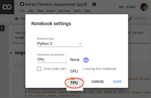
In the Colab menu, select Runtime > Change runtime type and then select TPU. In this code lab you will use a powerful TPU (Tensor Processing Unit) backed for hardware-accelerated training. Connection to the runtime will happen automatically on first execution, or you can use the "Connect" button in the upper-right corner.

Notebook execution

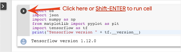
Execute cells one at a time by clicking on a cell and using Shift-ENTER. You can also run the entire notebook with Runtime > Run all

Table of contents

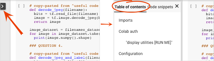
All notebooks have a table of contents. You can open it using the black arrow on the left.

Hidden cells

Some cells will only show their title. This is a Colab-specific notebook feature. You can double click on them to see the code inside but it is usually not very interesting. Typically support or visualization functions. You still need to run these cells for the functions inside to be defined.

Authentication

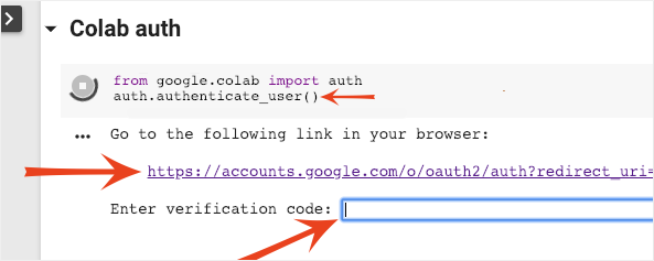
It is possible for Colab to access your private Google Cloud Storage buckets provided you authenticate with an authorized account. The code snippet above will trigger an authentication process.

3. [INFO] Neural network classifier 101

In a nutshell

If all the terms in bold in the next paragraph are already known to you, you can move to the next exercise. If your are just starting in deep learning then welcome, and please read on.

A neural network classifier is made of several layers of neurons. For image classification these can be dense or, more frequently, convolutional layers. They are typically activated with the relu activation function. The last layer uses as many neurons as there are classes and is activated with softmax. For classification, cross-entropy is the most commonly used loss function, comparing the one-hot encoded labels (i.e. correct answers) with probabilities predicted by the neural network. To minimize the loss, it is best to choose an optimizer with momentum, for example AdamOptimizer and train on batches of training images and labels.

For models built as a sequence of layers Keras offers the Sequential API. For example, an image classifier using three dense layers can be written in Keras as:

model = tf.keras.Sequential([
    tf.keras.layers.Flatten(input_shape=[192, 192, 3]),
    tf.keras.layers.Dense(500, activation="relu"),
    tf.keras.layers.Dense(50, activation="relu"),
    tf.keras.layers.Dense(5, activation='softmax') # classifying into 5 classes
])

# this configures the training of the model. Keras calls it "compiling" the model.
model.compile(
  optimizer='adam',
  loss= 'categorical_crossentropy',
  metrics=['accuracy']) # % of correct answers

# train the model
model.fit(dataset, ... )

Dense neural network

This is the simplest neural network for classifying images. It is made of "neurons" arranged in layers. The first layer processes input data and feeds its outputs into other layers. It is called "dense" because each neuron is connected to all the neurons in the previous layer.

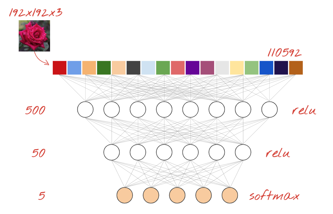
You can feed an image into such a network by flattening the RGB values of all of its pixels into a long vector and using it as inputs. It is not the best technique for image recognition but we will improve on it later.

Neurons, activations, RELU

A "neuron" computes a weighted sum of all of its inputs, adds a value called "bias" and feeds the result through a so called "activation function". The weights and bias are unknown at first. They will be initialized at random and "learned" by training the neural network on lots of known data.

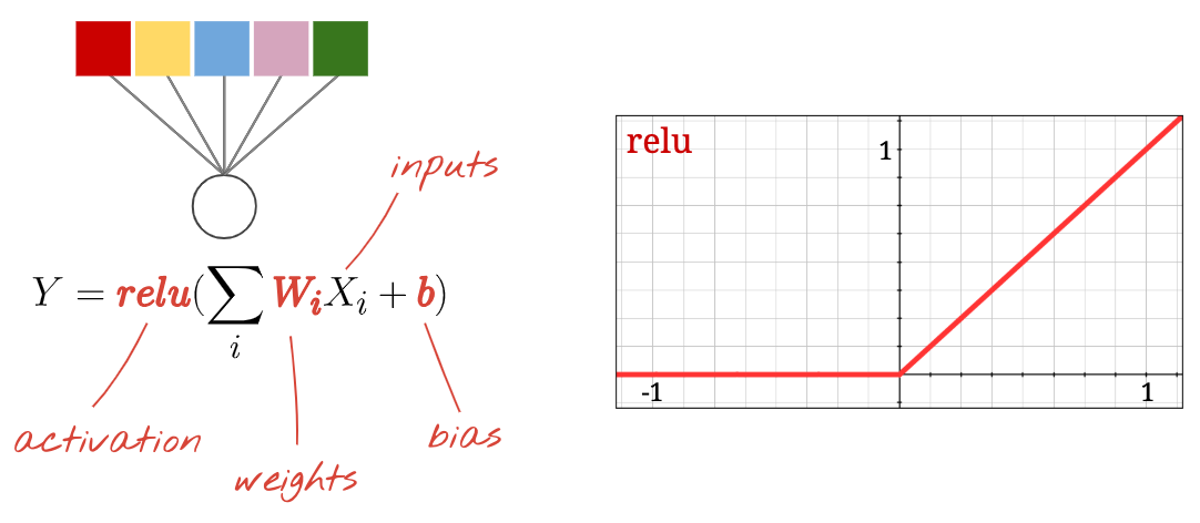
The most popular activation function is called RELU for Rectified Linear Unit. It is a very simple function as you can see on the graph above.

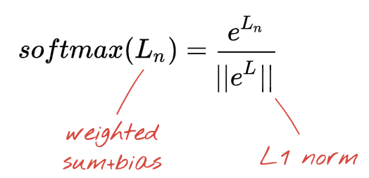
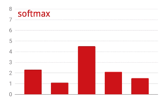
Softmax activation

The network above ends with a 5-neuron layer because we are classifying flowers into 5 categories (rose, tulip, dandelion, daisy, sunflower). Neurons in intermediate layers are activated using the classic RELU activation function. In the last layer though, we want to compute numbers between 0 and 1 representing the probability of this flower being a rose, a tulip and so on. For this, we will use an activation function called "softmax".

Applying softmax on a vector is done by taking the exponential of each element and then normalising the vector, typically using the L1 norm (sum of absolute values) so that the values add up to 1 and can be interpreted as probabilities.

Why is "softmax" called softmax? The exponential is a steeply increasing function. It will increase differences between the neuron outputs. Then, as you normalise the vector, the largest element, which dominates the norm, will be normalised to a value close to 1 while all the other elements will end up divided by a large value and normalised to something close to 0. The resulting vector clearly shows which is the winning class, the "max", but retains the original relative order of its values, hence the "soft".

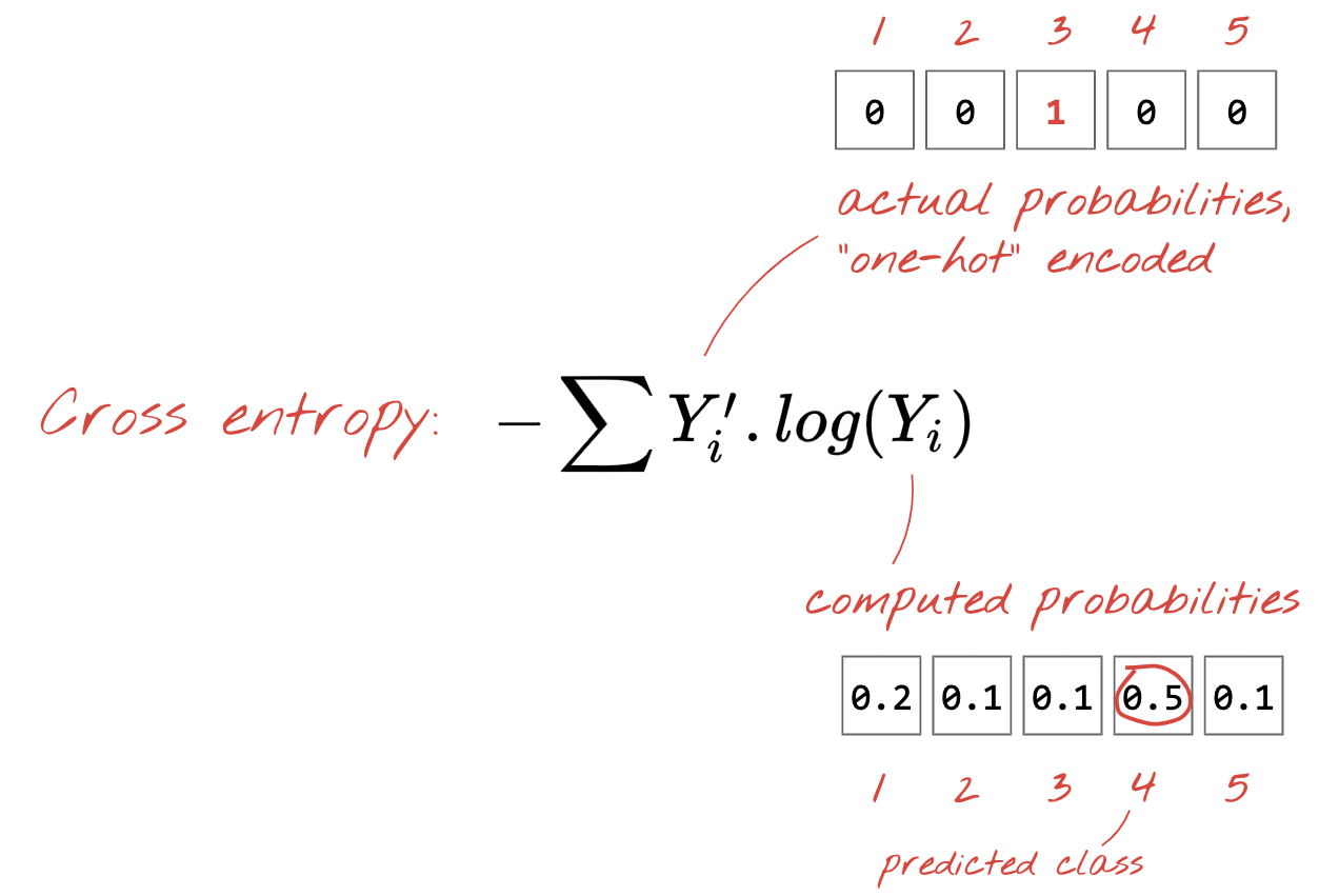
Cross-entropy loss

Now that our neural network produces predictions from input images, we need to measure how good they are, i.e. the distance between what the network tells us and the correct answers, often called "labels". Remember that we have correct labels for all the images in the dataset.

Any distance would work, but for classification problems the so-called "cross-entropy distance" is the most effective. We will call this our error or "loss" function:

"One-hot" encoding means that you represent the label "3) dandelion" by using a vector of 5 values, all zeros except for the the 3rd value which is 1. This vector represents a 100% probability of being a dandelion. Our neural network also outputs its predictions as a vector of 5 probability values. They are easy to compare.

Gradient descent

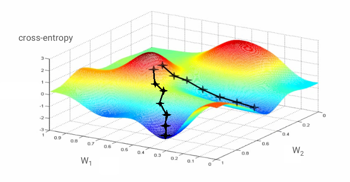
"Training" the neural network actually means using training images and labels to adjust weights and biases so as to minimise the cross-entropy loss function. Here is how it works.

The cross-entropy is a function of weights, biases, pixels of the training image and its known class.

If we compute the partial derivatives of the cross-entropy relatively to all the weights and all the biases we obtain a "gradient", computed for a given image, label, and present value of weights and biases. Remember that we can have millions of weights and biases so computing the gradient sounds like a lot of work. Fortunately, Tensorflow does it for us. The mathematical property of a gradient is that it points "up". Since we want to go where the cross-entropy is low, we go in the opposite direction. We update weights and biases by a fraction of the gradient. We then do the same thing again and again using the next batches of training images and labels, in a training loop. Hopefully, this converges to a place where the cross-entropy is minimal although nothing guarantees that this minimum is unique.

"Learning rate": You cannot update your weights and biases by the whole length of the gradient at each iteration. It would be like trying to get to the bottom of a valley while wearing seven-league boots. You would be jumping from one side of the valley to the other. To get to the bottom, you need to do smaller steps, i.e. use only a fraction of the gradient, typically in the 1/1000th range. This fraction is called the "learning rate".

Mini-batching and momentum

You can compute your gradient on just one example image and update the weights and biases immediately, but doing so on a batch of, for example, 128 images gives a gradient that better represents the constraints imposed by different example images and is therefore likely to converge towards the solution faster. The size of the mini-batch is an adjustable parameter.

This technique, sometimes called "stochastic gradient descent" has another, more pragmatic benefit: working with batches also means working with larger matrices and these are usually easier to optimise on GPUs and TPUs.

The convergence can still be a little chaotic though and it can even stop if the gradient vector is all zeros. Does that mean that we have found a minimum? Not always. A gradient component can be zero on a minimum or a maximum. With a gradient vector with millions of elements, if they are all zeros, the probability that every zero corresponds to a minimum and none of them to a maximum point is pretty small. In a space of many dimensions, saddle points are pretty common and we do not want to stop at them.

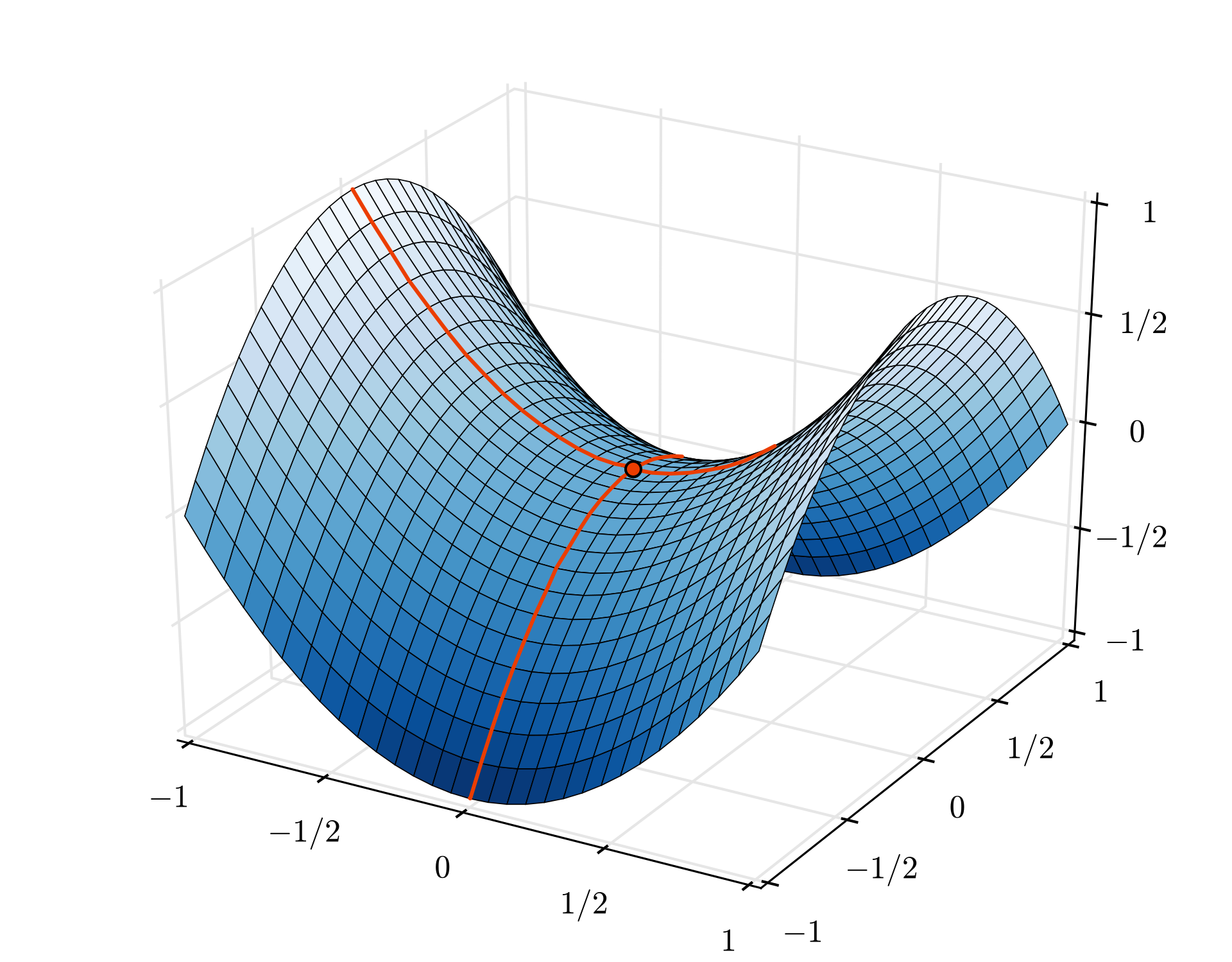
Illustration: a saddle point. The gradient is 0 but it is not a minimum in all directions. (Image attribution Wikimedia: By Nicoguaro - Own work, CC BY 3.0)

The solution is to add some momentum to the optimization algorithm so that it can sail past saddle points without stopping.

The Tensorflow library provides a whole range of optimizers, starting with tf.train.GradientDescentOptimizer. More advanced popular optimizers that have a built-in momentum are tf.train.RMSPropOptimizer or tf.train.AdamOptimizer.

Glossary

batch or mini-batch: training is always performed on batches of training data and labels. Doing so helps the algorithm converge. The "batch" dimension is typically the first dimension of data tensors. For example a tensor of shape [100, 192, 192, 3] contains 100 images of 192x192 pixels with three values per pixel (RGB).

cross-entropy loss: a special loss function often used in classifiers.

dense layer: a layer of neurons where each neuron is connected to all the neurons in the previous layer.

features: the inputs of a neural network are sometimes called "features". The art of figuring out which parts of a dataset (or combinations of parts) to feed into a neural network to get good predictions is called "feature engineering".

labels: another name for "classes" or correct answers in a supervised classification problem

learning rate: fraction of the gradient by which weights and biases are updated at each iteration of the training loop.

logits: the outputs of a layer of neurons before the activation function is applied are called "logits". The term comes from the "logistic function" a.k.a. the "sigmoid function" which used to be the most popular activation function. "Neuron outputs before logistic function" was shortened to "logits".

loss: the error function comparing neural network outputs to the correct answers

neuron: computes the weighted sum of its inputs, adds a bias and feeds the result through an activation function.

one-hot encoding: class 3 out of 5 is encoded as a vector of 5 elements, all zeros except the 3rd one which is 1.

relu: rectified linear unit. A popular activation function for neurons.

sigmoid: another activation function that used to be popular and is still useful in special cases.

softmax: a special activation function that acts on a vector, increases the difference between the largest component and all others, and also normalizes the vector to have a sum of 1 so that it can be interpreted as a vector of probabilities. Used as the last step in classifiers.

tensor: A "tensor" is like a matrix but with an arbitrary number of dimensions. A 1-dimensional tensor is a vector. A 2-dimensions tensor is a matrix. And then you can have tensors with 3, 4, 5 or more dimensions.

4. Transfer Learning

For an image classification problem, dense layers will probably not be enough. We have to learn about convolutional layers and the many ways you can arrange them.

But we can also take a shortcut! There are fully-trained convolutional neural networks available for download. It is possible to chop off their last layer, the softmax classification head, and replace it with your own. All the trained weights and biases stay as they are, you only retrain the softmax layer you add. This technique is called transfer learning and amazingly, it works as long as the dataset on which the neural net is pre-trained is "close enough" to yours.

Hands-on

Please open the following notebook, execute the cells (Shift-ENTER) and follow the instructions wherever you see a "WORK REQUIRED" label.

Keras Flowers transfer learning (playground).ipynb

Additional information

With transfer learning, you benefit from both advanced convolutional neural network architectures developed by top researchers and from pre-training on a huge dataset of images. In our case we will be transfer learning from a network trained on ImageNet, a database of images containing many plants and outdoors scenes, which is close enough to flowers.

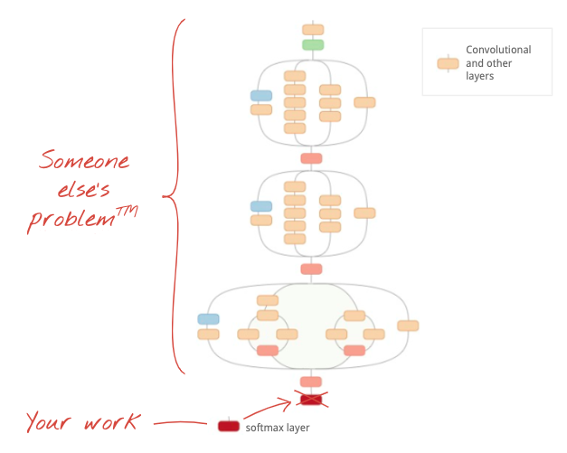
Illustration: using a complex convolutional neural network, already trained, as a black box, retraining the classification head only. This is transfer learning. We will see how these complicated arrangements of convolutional layers work later. For now, it is someone else's problem.

Transfer learning in Keras

In Keras, you can instantiate a pre-trained model from the tf.keras.applications.* collection. MobileNet V2 for example is a very good convolutional architecture that stays reasonable in size. By selecting include_top=False, you get the pre-trained model without its final softmax layer so that you can add your own:

pretrained_model = tf.keras.applications.MobileNetV2(input_shape=[*IMAGE_SIZE, 3], include_top=False)
pretrained_model.trainable = False

model = tf.keras.Sequential([
    pretrained_model,
    tf.keras.layers.Flatten(),
    tf.keras.layers.Dense(5, activation='softmax')
])

Also notice the pretrained_model.trainable = False setting. It freezes the weights and biases of the pre-trained model so that you train your softmax layer only. This typically involves relatively few weights and can be done quickly and without necessitating a very large dataset. However if you do have lots of data, transfer learning can work even better with pretrained_model.trainable = True. The pre-trained weights then provide excellent initial values and can still be adjusted by the training to better fit your problem.

Finally, notice the Flatten() layer inserted before your dense softmax layer. Dense layers work on flat vectors of data but we do not know if that is what the pretrained model returns. That's why we need to flatten. In the next chapter, as we dive into convolutional architectures, we will explain the data format returned by convolutional layers.

You should get close to 75% accuracy with this approach.

Solution

Here is the solution notebook. You can use it if you are stuck.

Keras Flowers transfer learning (solution).ipynb

What we've covered

• 🤔 How to write a classifier in Keras
• 🤓 configured with a softmax last layer, and cross-entropy loss
• 😈 Transfer learning
• 🤔 Training your first model
• 🧐 Following its loss and accuracy during training

Please take a moment to go through this checklist in your head.

5. Congratulations!

You can now build a Keras model. Please continue to the next lab to learn how to assemble convolutional layers.

• TPU-speed data pipelines: tf.data.Dataset and TFRecords
• [THIS LAB] Your first Keras model, with transfer learning
• Convolutional neural networks, with Keras and TPUs
• Modern convnets, squeezenet, Xception, with Keras and TPUs

TPUs in practice

TPUs and GPUs are available on Cloud AI Platform:

• On Deep Learning VMs
• In AI Platform Notebooks
• In AI Platform Training jobs

Finally, we love feedback. Please tell us if you see something amiss in this lab or if you think it should be improved. Feedback can be provided through GitHub issues [ feedback link].

The author: Martin Görner Twitter: @martin_gorner

www.tensorflow.org