
1. Overview
This lab will walk you through various tools in AI Platform Notebooks for exploring your data and prototyping ML models.
What you learn
You'll learn how to:
- Create and customize an AI Platform Notebooks instance
- Track your notebooks code with git, directly integrated into AI Platform Notebooks
- Use the What-If Tool within your notebook
The total cost to run this lab on Google Cloud is about $1. Full details on AI Platform Notebooks pricing can be found here.
2. Create an AI Platform Notebooks instance
You'll need a Google Cloud Platform project with billing enabled to run this codelab. To create a project, follow the instructions here.
Step 2: Enable the Compute Engine API
Navigate to Compute Engine and select Enable if it isn't already enabled. You'll need this to create your notebook instance.
Step 3: Create a notebook instance
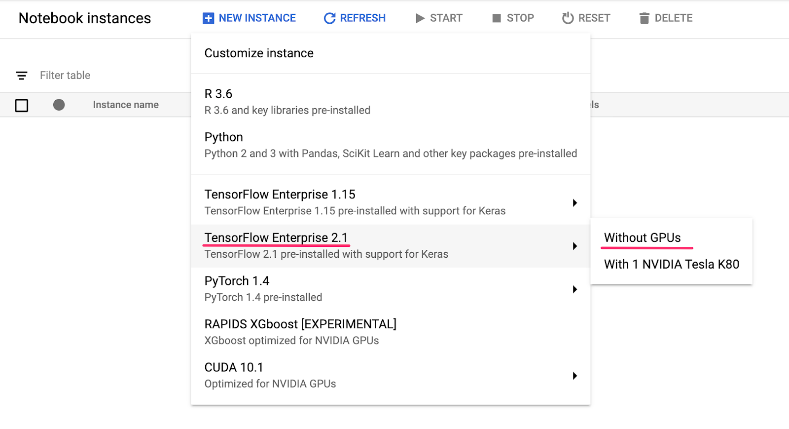
Navigate to AI Platform Notebooks section of your Cloud Console and click New Instance. Then select the latest TensorFlow 2 Enterprise instance type without GPUs:
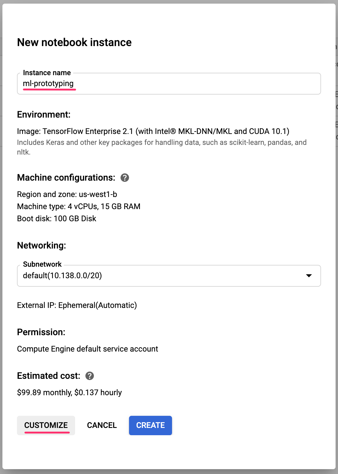
Give your instance a name or use the default. Then we'll explore the customization options. Click the Customize button:
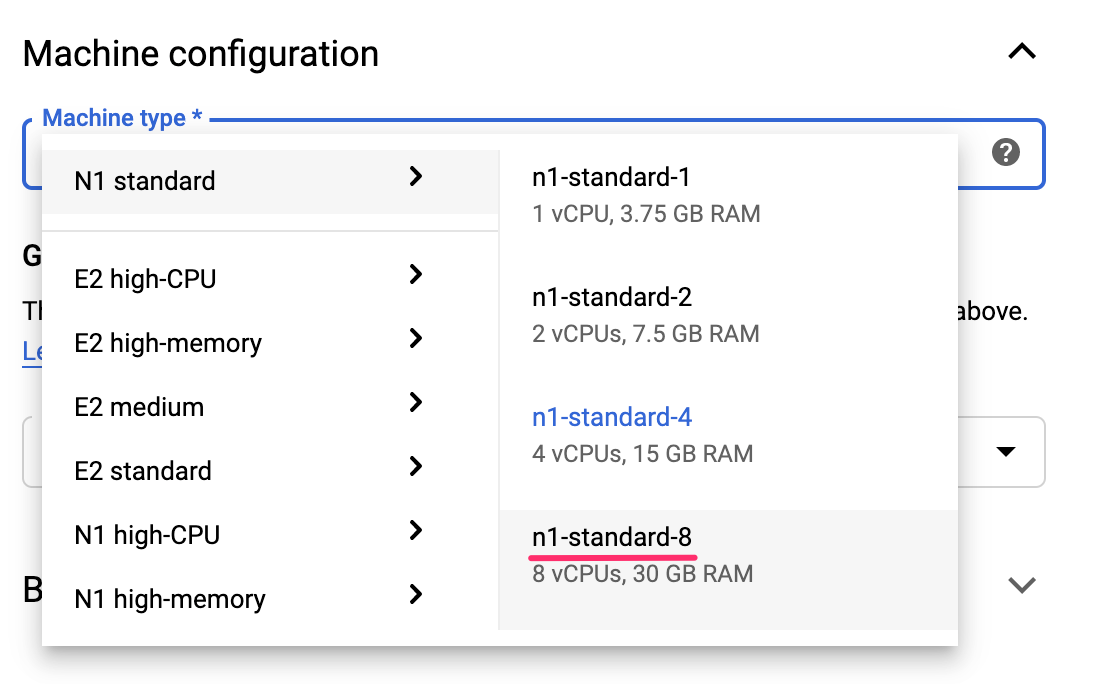
AI Platform Notebooks has many different customization options, including: the region your instance is deployed in, the image type, machine size, number of GPUs, and more. We'll use the defaults for region and environment. For machine configuration, we'll use an n1-standard-8 machine:
We won't add any GPUs, and we'll use the defaults for boot disk, networking, and permission. Select Create to create your instance. This will take a few minutes to complete.
Once the instance has been created you'll see a green checkmark next to it in the Notebooks UI. Select Open JupyterLab to open your instance and start prototyping:

When you open the instance, create a new directory called codelab. This is the directory we'll be working from throughout this lab:

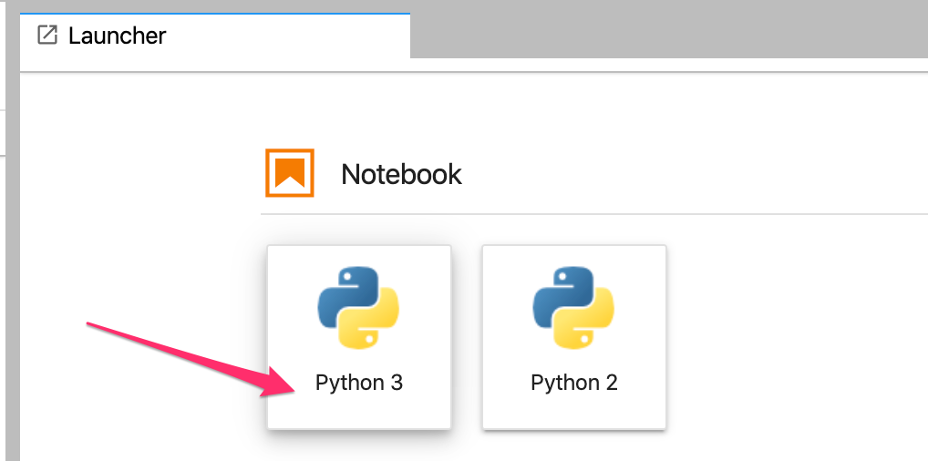
Click into your newly created codelab directory by double-clicking on it and then select Python 3 notebook from the launcher:
Rename the notebook to demo.ipynb, or whatever name you'd like to give it.
Step 4: Import Python packages
Create a new cell in the notebook and import the libraries we'll be using in this codelab:
import pandas as pd
import tensorflow as tf
from tensorflow.keras import Sequential
from tensorflow.keras.layers import Dense

import numpy as np
import json

from sklearn.model_selection import train_test_split
from sklearn.utils import shuffle
from google.cloud import bigquery
from witwidget.notebook.visualization import WitWidget, WitConfigBuilder
3. Connect BigQuery data to your notebook
BigQuery, Google Cloud's big data warehouse, has made many datasets publicly available for your exploration. AI Platform Notebooks support direct integration with BigQuery without requiring authentication.
For this lab, we'll be using the natality dataset. This contains data on nearly every birth in the US over a 40 year time period, including the birth weight of the child, and demographic information on the baby's parents. We'll be using a subset of the features to predict a baby's birth weight.
Step 1: Download BigQuery data to our notebook
We'll be using the Python client library for BigQuery to download the data into a Pandas DataFrame. The original dataset is 21GB and contains 123M rows. To keep things simple we'll only be using 10,000 rows from the dataset.
Construct the query and preview the resulting DataFrame with the following code. Here we're getting 4 features from the original dataset, along with baby weight (the thing our model will predict). The dataset goes back many years but for this model we'll use only data from after 2000:
query="""
SELECT
  weight_pounds,
  is_male,
  mother_age,
  plurality,
  gestation_weeks
FROM
  publicdata.samples.natality
WHERE year > 2000
LIMIT 10000
"""
df = bigquery.Client().query(query).to_dataframe()
df.head()
To get a summary of the numeric features in our dataset, run:
df.describe()
This shows the mean, standard deviation, minimum, and other metrics for our numeric columns. Finally, let's get some data on our boolean column indicating the baby's gender. We can do this with Pandas value_counts method:
df['is_male'].value_counts()
Looks like the dataset is nearly balanced 50/50 by gender.
Step 2: Prepare the dataset for training
Now that we've downloaded the dataset to our notebook as a Pandas DataFrame, we can do some pre-processing and split it into training and test sets.
First, let's drop rows with null values from the dataset and shuffle the data:
df = df.dropna()
df = shuffle(df, random_state=2)
Next, extract the label column into a separate variable and create a DataFrame with only our features. Since is_male is a boolean, we'll convert it to an integer so that all inputs to our model are numeric:
labels = df['weight_pounds']
data = df.drop(columns=['weight_pounds'])
data['is_male'] = data['is_male'].astype(int)
Now if you preview our dataset by running data.head(), you should see the four features we'll be using for training.
4. Initialize git
AI Platform Notebooks has a direct integration with git, so that you can do version control directly within your notebook environment. This supports committing code right in the notebook UI, or via the Terminal available in JupyterLab. In this section we'll initialize a git repository in our notebook and make our first commit via the UI.
Step 1: Initialize a git repository
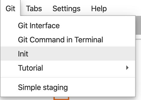
From your codelab directory, select Git and then Init from the top menu bar in JupyterLab:
When it asks if you want to make this directory a Git Repo, select Yes. Then select the Git icon on the left sidebar to see the status of your files and commits:

Step 2: Make your first commit
In this UI, you can add files to a commit, see file diffs (we'll get to that later), and commit your changes. Let's start by committing the notebook file we just added.
Check the box next to your demo.ipynb notebook file to stage it for the commit (you can ignore the .ipynb_checkpoints/ directory). Enter a commit message in the text box and then click on the check mark to commit your changes:

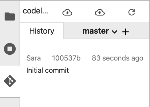
Enter your name and email when prompted. Then go back to the History tab to see your first commit:
Note that the screenshots might not match your UI exactly, due to updates since this lab was published.
5. Build and train a TensorFlow model
We'll use the BigQuery natality dataset we've downloaded to our notebook to build a model that predicts baby weight. In this lab we'll be focusing on the notebook tooling, rather than the accuracy of the model itself.
Step 1: Split your data into train and test sets
We'll use the Scikit Learn train_test_split utility to split our data before building our model:
x,y = data,labels
x_train,x_test,y_train,y_test = train_test_split(x,y)
Now we're ready to build our TensorFlow model!
Step 2: Build and train the TensorFlow model
We'll be building this model using the tf.keras Sequential model API, which lets us define our model as a stack of layers. All the code we need to build our model is here:
model = Sequential([
    Dense(64, activation='relu', input_shape=(len(x_train.iloc[0]),)),
    Dense(32, activation='relu'),
    Dense(1)]
)
Then we'll compile our model so we can train it. Here we'll choose the model's optimizer, loss function, and metrics we'd like the model to log during training. Since this is a regression model (predicting a numerical value), we're using mean squared error instead of accuracy as our metric:
model.compile(optimizer=tf.keras.optimizers.RMSprop(),
              loss=tf.keras.losses.MeanSquaredError(),
              metrics=['mae', 'mse'])
You can use Keras's handy model.summary() function to see the shape and number of trainable parameters of your model at each layer.
Now we're ready to train our model. All we need to do is call the fit() method, passing it our training data and labels. Here we'll use the optional validation_split parameter, which will hold a portion of our training data to validate the model at each step. Ideally you want to see training and validation loss both decreasing. But remember that in this example we're more focused on model and notebook tooling rather than model quality:
model.fit(x_train, y_train, epochs=10, validation_split=0.1)
Step 3: Generate predictions on test examples
To see how our model is performing, let's generate some test predictions on the first 10 examples from our test dataset.
num_examples = 10
predictions = model.predict(x_test[:num_examples])
And then we'll iterate over our model's predictions, comparing them to the actual value:
for i in range(num_examples):
    print('Predicted val: ', predictions[i][0])
    print('Actual val: ',y_test.iloc[i])
    print()
Step 4: Use git diff and commit your changes
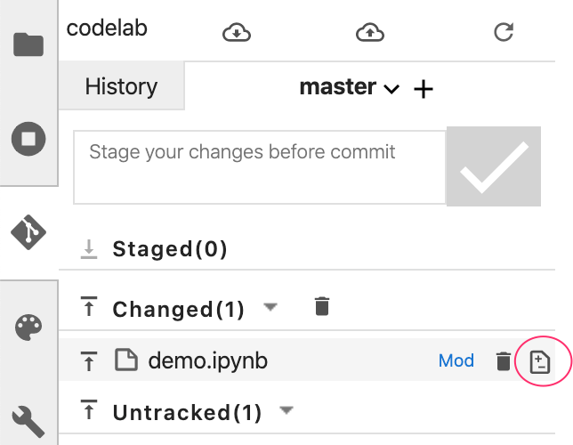
Now that you've made some changes to the notebook, you can try out the git diff feature available in the Notebooks git UI. The demo.ipynb notebook should now be under the "Changed" section in the UI. Hover over the filename and click on the diff icon:
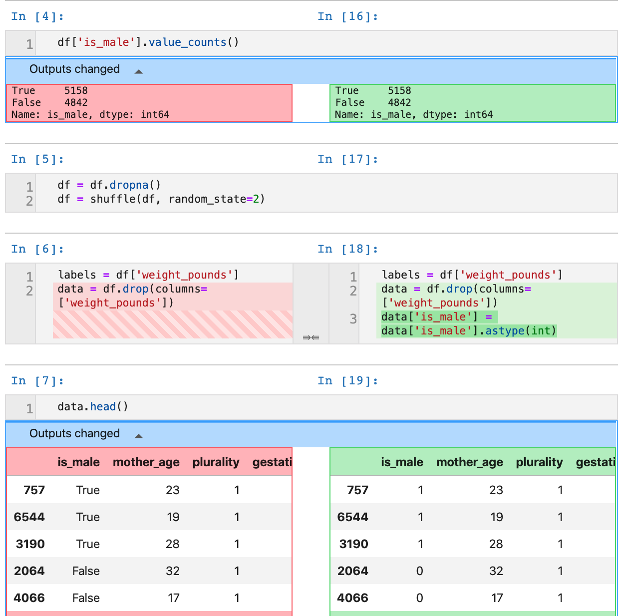
With that you should be able to see a diff of your changes, like the following:
This time we'll commit our changes via the command line using Terminal. From the Git menu in the JupyterLab top menu bar, select Git Command in Terminal. If you have the git tab of your left sidebar open while you run the commands below, you'll be able to see your changes reflected in the git UI.
In your new terminal instance, run the following to stage your notebook file for commit:
git add demo.ipynb
And then run the following to commit your changes (you can use whatever commit message you'd like):
git commit -m "Build and train TF model"
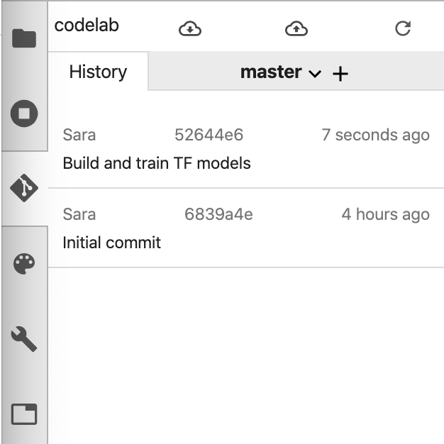
Then you should see your latest commit in the history:
6. Use the What-If Tool directly from your notebook
The What-If Tool is an interactive visual interface designed to help you visualize your datasets and better understand the output of your ML models. It is an open source tool created by the PAIR team at Google. While it works with any type of model, it has some features built exclusively for Cloud AI Platform.
The What-If Tool comes pre-installed in Cloud AI Platform Notebooks instances with TensorFlow. Here we'll use it to see how our model is performing overall and inspect its behavior on data points from our test set.
Step 1: Prepare data for the What-If Tool
To make the most of the What-If Tool, we'll send it examples from our test set along with the ground truth labels for those examples (y_test). That way we can compare what our model predicted to the ground truth. Run the line of code below to create a new DataFrame with our test examples and their labels:
wit_data = pd.concat([x_test, y_test], axis=1)
In this lab, we'll be connecting the What-If Tool to the model we've just trained in our notebook. In order to do that, we need to write a function that the tool will use to run these test data points to our model:
def custom_predict(examples_to_infer):
    preds = model.predict(examples_to_infer)
    return preds
Step 2: Instantiate the What-If Tool
We'll instantiate the What-If Tool by passing it 500 examples from the concatenated test dataset + ground truth labels we just created. We create an instance of WitConfigBuilder to set up the tool, passing it our data, the custom predict function we defined above, along with our target (the thing we're predicting), and the model type:
config_builder = (WitConfigBuilder(wit_data[:500].values.tolist(), data.columns.tolist() + ['weight_pounds'])
  .set_custom_predict_fn(custom_predict)
  .set_target_feature('weight_pounds')
  .set_model_type('regression'))
WitWidget(config_builder, height=800)
You should see something like this when the What-If Tool loads:
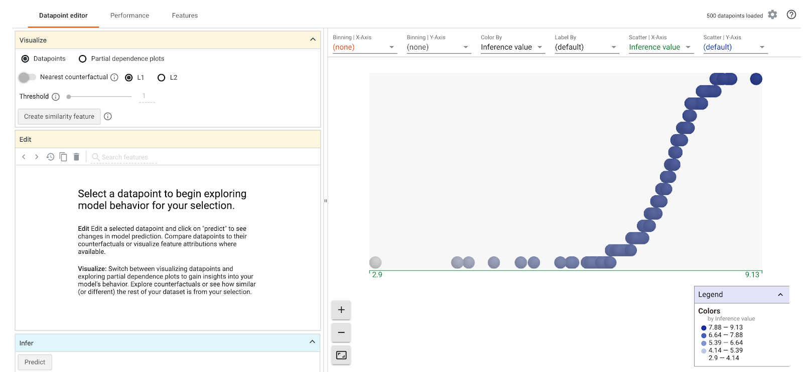
On the x-axis, you can see your test data points spread out by the model's predicted weight value, weight_pounds.
Step 3: Explore model behavior with the What-If Tool
There are lots of cool things you can do with the What-If Tool. We'll explore just a few of them here. First, let's look at the datapoint editor. You can select any data point to see its features, and change the feature values. Start by clicking on any data point:
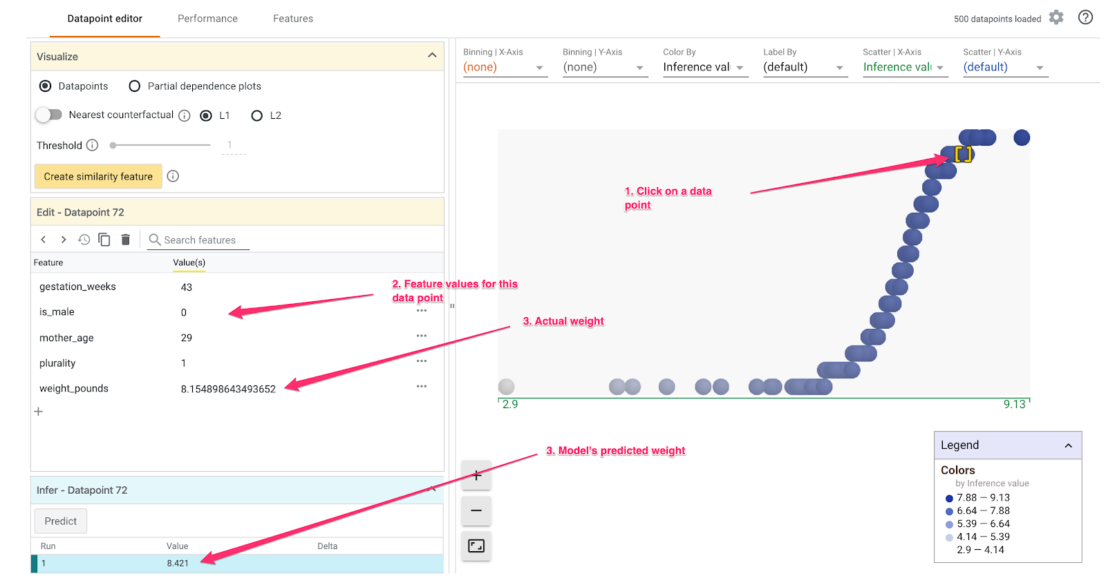
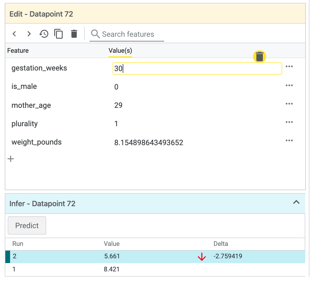
On the left you'll see the feature values for the data point you've selected. You can also compare that data point's ground truth label with the value predicted by the model. In the left sidebar, you can also change feature values and re-run model prediction to see the effect this change had on your model. For example, we can change gestation_weeks to 30 for this data point by double-clicking on it an re-run prediction:
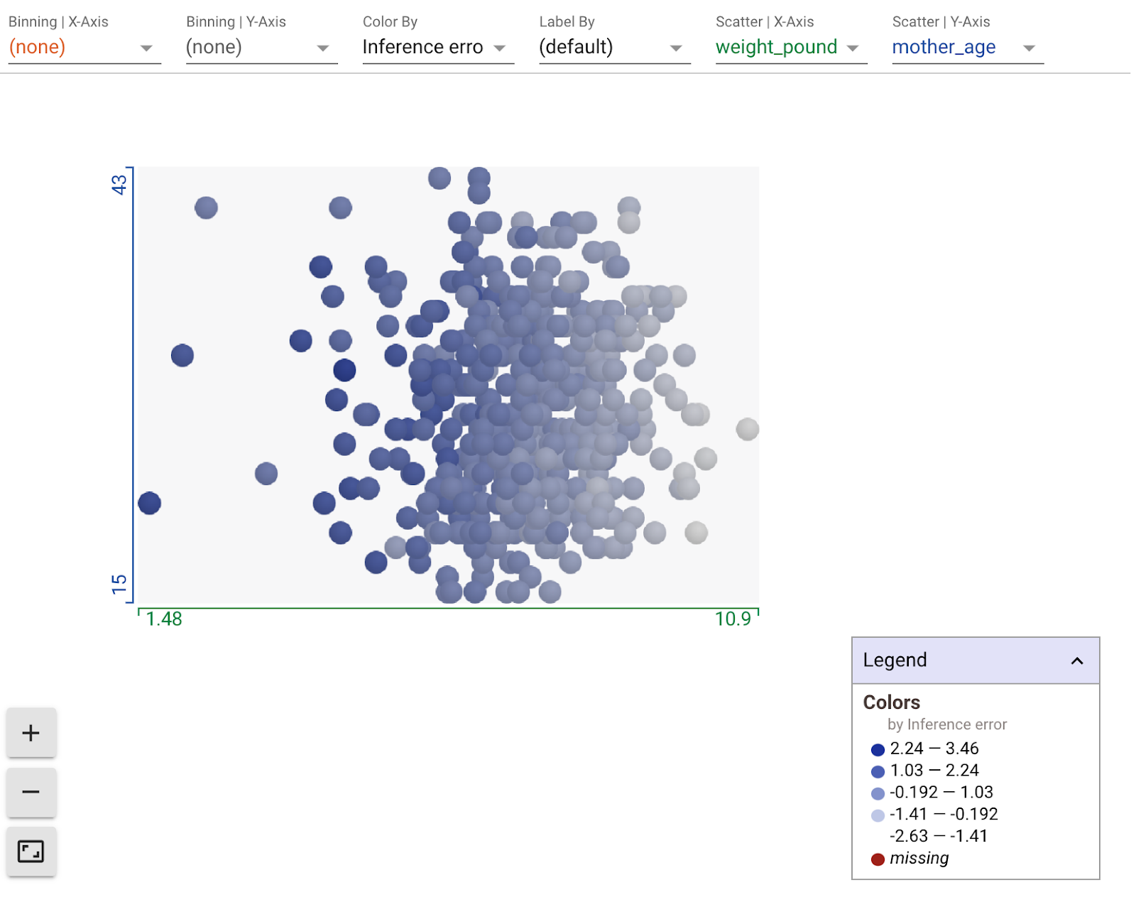
Using the dropdown menus in the plot section of the What-If Tool, you can create all sorts of custom visualizations. For example, here's a chart with the models' predicted weight on the x-axis, the age of the mother on the y-axis, and points colored by their inference error (darker means a higher difference between predicted and actual weight). Here it looks like as weight decreases, the model's error increases slightly:
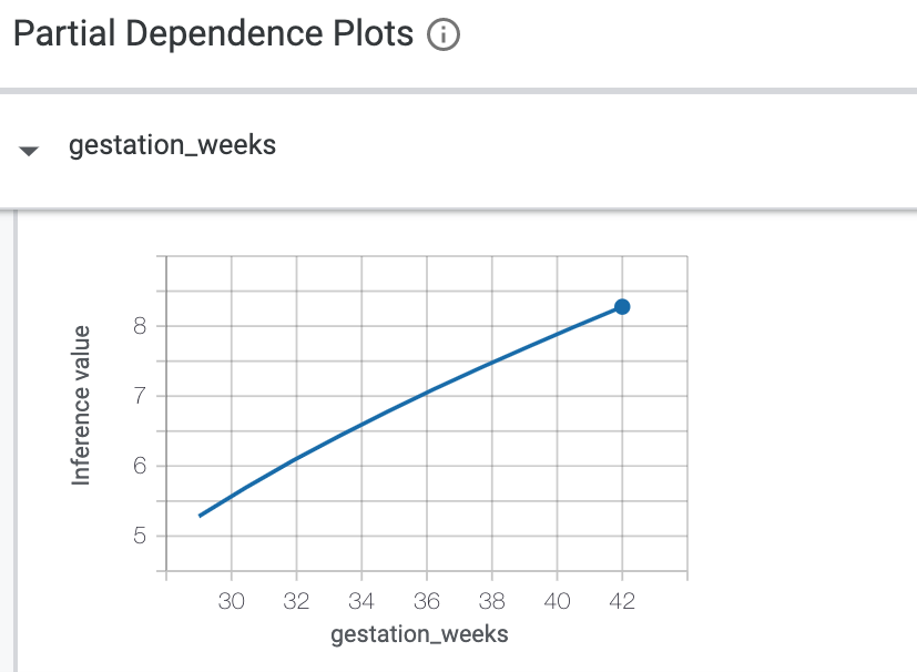
Next, check the Partial dependence plots button on the left. This shows how each feature influences the model's prediction. For example, as gestation time increases, our model's predicted baby weight also increases:
For more exploration ideas with the What-If Tool, check the links at the beginning of this section.
7. Optional: connect your local git repo to GitHub
Finally, we'll learn how to connect the git repo in our notebook instance to a repo in our GitHub account. If you'd like to do this step, you'll need a GitHub account.
Step 1: Create a new repo on GitHub
In your GitHub account, create a new repository. Give it a name and a description, decide if you'd like it to be public, and select Create repository (you don't need to initialize with a README). On the next page, you'll follow the instructions for pushing an existing repository from the command line.
Open a Terminal window, and add your new repository as a remote. Replace username in the repo URL below with your GitHub username, and your-repo with the name of the one you just created:
git remote add origin git@github.com:username/your-repo.git
Step 2: Authenticate to GitHub in your notebooks instance
Next you'll need to authenticate to GitHub from within your notebook instance. This process varies depending on whether you have two-factor authentication enabled on GitHub.
If you're not sure where to start, follow the steps in the GitHub documentation to create an SSH key and then add the new key to GitHub.
Step 3: Ensure you've correctly linked your GitHub repo
To make sure you've set things up correctly, run git remote -v in your terminal. You should see your new repository listed as a remote. Once you see the URL of your GitHub repo and you've authenticated to GitHub from your notebook, you're ready to push directly to GitHub from your notebook instance.
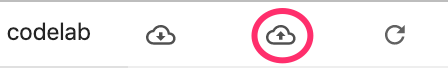
To sync your local notebook git repo with your newly created GitHub repo, click the cloud upload button at the top of the Git sidebar:
Refresh your GitHub repository, and you should see your notebook code with your previous commits! If others have access to your GitHub repo and you'd like to pull down the latest changes to your notebook, click the cloud download icon to sync those changes.
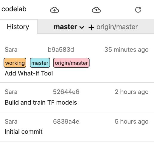
On the History tab of the Notebooks git UI, you can see if your local commits are synced with GitHub. In this example, origin/master corresponds with our repo on GitHub:
Whenever you make new commits, just click the cloud upload button again to push those changes to your GitHub repo.
8. Congrats!
You've done a lot in this lab 👏👏👏
To recap, you've learned how to:
- Create an customize an AI Platform Notebook instance
- Initialize a local git repo in that instance, add commits via the git UI or command line, view git diffs in the Notebook git UI
- Build and train a simple TensorFlow 2 model
- Use the What-If Tool within your Notebook instance
- Connect your Notebook git repo to an external repository on GitHub
9. Cleanup
If you'd like to continue using this notebook, it is recommended that you turn it off when not in use. From the Notebooks UI in your Cloud Console, select the notebook and then select Stop:
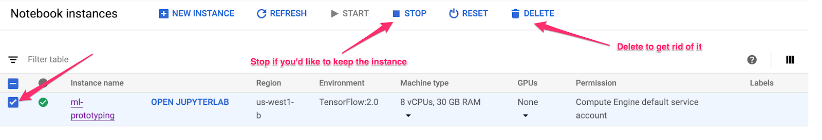
If you'd like to delete all resources you've created in this lab, simply delete the notebook instance instead of stopping it.
Using the Navigation menu in your Cloud Console, browse to Storage and delete both buckets you created to store your model assets.