מציגים מסווגי בטיחות גמישים עם Gemma

1. סקירה כללית

ה-Codelab הזה מדגים איך ליצור מסווג טקסט בהתאמה אישית באמצעות כוונון יעיל של פרמטרים (PET). במקום לבצע כוונון עדין של המודל כולו, שיטות PET מעדכנות רק כמות קטנה של פרמטרים, ולכן קל ומהיר יחסית לאמן את המודל. בנוסף, קל יותר למודל ללמוד התנהגויות חדשות עם כמות קטנה יחסית של נתוני אימון. המתודולוגיה מתוארת בפירוט במאמר Towards Agile Text Classifiers for Everyone, שבו מוסבר איך אפשר להשתמש בטכניקות האלה במגוון משימות שקשורות לבטיחות, ולהשיג ביצועים מתקדמים עם כמה מאות דוגמאות לאימון בלבד.

ב-codelab הזה נעשה שימוש בשיטת PET של LoRA ובמודל Gemma הקטן יותר (gemma_instruct_2b_en), כי אפשר להריץ אותו מהר יותר וביעילות רבה יותר. ב-Colab מוסבר איך להטמיע נתונים, לעצב אותם בשביל מודל LLM, לאמן משקלים של LoRA ואז להעריך את התוצאות. ב-codelab הזה מתאמנים על מערך הנתונים ETHOS, מערך נתונים שזמין לציבור לזיהוי של דברי שטנה, שנבנה על סמך תגובות ב-YouTube וב-Reddit. כשהמודל אומן על 200 דוגמאות בלבד (רבע ממערך הנתונים), הוא השיג F1: 0.80 ו-ROC-AUC: 0.78, קצת מעל ה-SOTA שדווח כרגע בטבלת המובילים (בזמן הכתיבה, 15 בפברואר 2024). כשהמודל אומן על 800 הדוגמאות המלאות, הוא השיג ציון F1 של 83.74 וציון ROC-AUC של 88.17. מודלים גדולים יותר, כמו gemma_instruct_7b_en, בדרך כלל יניבו ביצועים טובים יותר, אבל עלויות האימון וההפעלה שלהם גם גבוהות יותר.

אזהרה: ב-codelab הזה מפתחים מסווג בטיחות לזיהוי של דברי שטנה, ולכן הדוגמאות וההערכה של התוצאות מכילים שפה נוראית.

2. התקנה והגדרה

כדי להשתמש ב-codelab הזה, תצטרכו גרסה עדכנית של keras (3), ‏ keras-nlp (0.8.0) וחשבון Kaggle כדי להוריד את מודל הבסיס.

!pip install -q -U keras-nlp
!pip install -q -U keras

כדי להתחבר ל-Kaggle, אפשר לשמור את קובץ פרטי הכניסה kaggle.json במיקום ~/.kaggle/kaggle.json או להריץ את הפקודה הבאה בסביבת Colab:

import kagglehub

kagglehub.login()

ה-codelab הזה נבדק באמצעות Tensorflow כ-Keras backend, אבל אפשר להשתמש ב-Tensorflow, ב-Pytorch או ב-JAX:

import os

os.environ["KERAS_BACKEND"] = "tensorflow"

3. טעינה של מערך הנתונים ETHOS

בקטע הזה נטען את מערך הנתונים שעליו נאמן את המסווג שלנו, ונבצע בו עיבוד מקדים כדי ליצור ממנו קבוצת אימון וקבוצת נתונים לבדיקה. תשתמשו במערך הנתונים הפופולרי למחקר ETHOS, שנאסף כדי לזהות דברי שטנה ברשתות החברתיות. מידע נוסף על אופן איסוף מערך הנתונים מופיע במאמר ETHOS: an Online Hate Speech Detection Dataset.

import pandas as pd

gh_root = 'https://raw.githubusercontent.com'
gh_repo = 'intelligence-csd-auth-gr/Ethos-Hate-Speech-Dataset'
gh_path = 'master/ethos/ethos_data/Ethos_Dataset_Binary.csv'
data_url = f'{gh_root}/{gh_repo}/{gh_path}'

df = pd.read_csv(data_url, delimiter=';')
df['hateful'] = (df['isHate'] >= df['isHate'].median()).astype(int)

# Shuffle the dataset.
df = df.sample(frac=1, random_state=32)

# Split into train and test.
df_train, df_test = df[:800],  df[800:]

# Display a sample of the data.
df.head(5)[['hateful', 'comment']]

יוצג לכם משהו דומה לזה:

	תווית	תגובה
0	0	You said he but still not convinced this is a ...
1	0	well, looks like its time to have another child.
2	0	What if we send every men to mars to start a n...
3	1	It doesn't matter if you're black or white, ...
4	0	Who ever disliked this video should be ashamed...

4. הורדה ויצירת מופע של המודל

כמו שמתואר במסמכי התיעוד, אפשר להשתמש במודל Gemma בקלות בדרכים רבות. כך עושים זאת באמצעות Keras:

import keras
import keras_nlp

# For reproducibility purposes.
keras.utils.set_random_seed(1234)

# Download the model from Kaggle using Keras.
model = keras_nlp.models.GemmaCausalLM.from_preset('gemma_instruct_2b_en')

# Set the sequence length to a small enough value to fit in memory in Colab.
model.preprocessor.sequence_length = 128

כדי לבדוק שהמודל פועל, אפשר ליצור טקסט:

model.generate('Question: what is the capital of France? ', max_length=32)

5. עיבוד מקדים של טקסט וטוקנים של מפרידים

כדי לעזור למודל להבין טוב יותר את הכוונה שלנו, אפשר לבצע עיבוד מקדים של הטקסט ולהשתמש בטוקנים של מפרידים. כך יש סיכוי נמוך יותר שהמודל ייצור טקסט שלא מתאים לפורמט הצפוי. לדוגמה, אפשר לנסות לבקש מהמודל לסווג את הסנטימנט על ידי כתיבת הנחיה כזו:

Classify the following text into one of the following classes:[Positive,Negative]

Text: you look very nice today
Classification:

במקרה כזה, יכול להיות שהמודל יפיק את מה שחיפשתם ויכול להיות שלא. לדוגמה, אם הטקסט מכיל תווי שורה חדשה, סביר להניח שתהיה לכך השפעה שלילית על ביצועי המודל. גישה חזקה יותר היא להשתמש בטוקנים של מפרידים. ההנחיה תהפוך ל:

Classify the following text into one of the following classes:[Positive,Negative]
<separator>
Text: you look very nice today
<separator>
Prediction:

אפשר להשתמש בפונקציה שמבצעת עיבוד מקדים של הטקסט כדי להשיג הפשטה:

def preprocess_text(
    text: str,
    labels: list[str],
    instructions: str,
    separator: str,
) -> str:
  prompt = f'{instructions}:[{",".join(labels)}]'
  return separator.join([prompt, f'Text:{text}', 'Prediction:'])

עכשיו, אם מריצים את הפונקציה באמצעות אותה הנחיה ואותו טקסט כמו קודם, אמור להתקבל אותו פלט:

text = 'you look very nice today'

prompt = preprocess_text(
    text=text,
    labels=['Positive', 'Negative'],
    instructions='Classify the following text into one of the following classes',
    separator='\n<separator>\n',
)

print(prompt)

הפלט שיתקבל:

Classify the following text into one of the following classes:[Positive,Negative]
<separator>
Text:well, looks like its time to have another child
<separator>
Prediction:

6. עיבוד תמונה (Post Processing) של הפלט

הפלט של המודל הוא אסימונים עם הסתברויות שונות. בדרך כלל, כדי ליצור טקסט, בוחרים מתוך כמה מהטוקנים הסבירים ביותר ומרכיבים משפטים, פסקאות או אפילו מסמכים מלאים. עם זאת, לצורך סיווג, מה שחשוב באמת הוא אם המודל מאמין שהסבירות ל-Positive גבוהה יותר מאשר ל-Negative או להיפך.

בהינתן המודל שיצרתם מופע שלו קודם לכן, כך תוכלו לעבד את הפלט שלו כדי לקבל את ההסתברויות הבלתי תלויות לכך שהטוקן הבא הוא Positive או Negative:

import numpy as np


def compute_output_probability(
    model: keras_nlp.models.GemmaCausalLM,
    prompt: str,
    target_classes: list[str],
) -> dict[str, float]:
  # Shorthands.
  preprocessor = model.preprocessor
  tokenizer = preprocessor.tokenizer

  # NOTE: If a token is not found, it will be considered same as "<unk>".
  token_unk = tokenizer.token_to_id('<unk>')

  # Identify the token indices, which is the same as the ID for this tokenizer.
  token_ids = [tokenizer.token_to_id(word) for word in target_classes]

  # Throw an error if one of the classes maps to a token outside the vocabulary.
  if any(token_id == token_unk for token_id in token_ids):
    raise ValueError('One of the target classes is not in the vocabulary.')

  # Preprocess the prompt in a single batch. This is done one sample at a time
  # for illustration purposes, but it would be more efficient to batch prompts.
  preprocessed = model.preprocessor.generate_preprocess([prompt])

  # Identify output token offset.
  padding_mask = preprocessed["padding_mask"]
  token_offset = keras.ops.sum(padding_mask) - 1

  # Score outputs, extract only the next token's logits.
  vocab_logits = model.score(
      token_ids=preprocessed["token_ids"],
      padding_mask=padding_mask,
  )[0][token_offset]

  # Compute the relative probability of each of the requested tokens.
  token_logits = [vocab_logits[ix] for ix in token_ids]
  logits_tensor = keras.ops.convert_to_tensor(token_logits)
  probabilities = keras.activations.softmax(logits_tensor)

  return dict(zip(target_classes, probabilities.numpy()))

כדי לבדוק את הפונקציה, מריצים אותה עם ההנחיה שיצרתם קודם:

compute_output_probability(
    model=model,
    prompt=prompt,
    target_classes=['Positive', 'Negative'],
)

הפלט שיתקבל ייראה בערך כך:

{'Positive': 0.99994016, 'Negative': 5.984089e-05}

7. עוטפים את הכול כסיווג

כדי להקל על השימוש, אפשר לאגד את כל הפונקציות שיצרתם לסיווג יחיד שדומה ל-sklearn, עם פונקציות מוכרות וקלות לשימוש כמו predict() ו-predict_score().

import dataclasses


@dataclasses.dataclass(frozen=True)
class AgileClassifier:
  """Agile classifier to be wrapped around a LLM."""

  # The classes whose probability will be predicted.
  labels: tuple[str, ...]

  # Provide default instructions and control tokens, can be overridden by user.
  instructions: str = 'Classify the following text into one of the following classes'
  separator_token: str = '<separator>'
  end_of_text_token: str = '<eos>'

  def encode_for_prediction(self, x_text: str) -> str:
    return preprocess_text(
        text=x_text,
        labels=self.labels,
        instructions=self.instructions,
        separator=self.separator_token,
    )

  def encode_for_training(self, x_text: str, y: int) -> str:
    return ''.join([
        self.encode_for_prediction(x_text),
        self.labels[y],
        self.end_of_text_token,
    ])

  def predict_score(
      self,
      model: keras_nlp.models.GemmaCausalLM,
      x_text: str,
  ) -> list[float]:
    prompt = self.encode_for_prediction(x_text)
    token_probabilities = compute_output_probability(
        model=model,
        prompt=prompt,
        target_classes=self.labels,
    )
    return [token_probabilities[token] for token in self.labels]

  def predict(
      self,
      model: keras_nlp.models.GemmaCausalLM,
      x_eval: str,
  ) -> int:
    return np.argmax(self.predict_score(model, x_eval))


agile_classifier = AgileClassifier(labels=('Positive', 'Negative'))

8. כוונון עדין של מודלים

‫LoRA הוא קיצור של Low-Rank Adaptation. זו טכניקת כוונון עדין שאפשר להשתמש בה כדי לבצע כוונון עדין של מודלים גדולים של שפה בצורה יעילה. אפשר לקרוא מידע נוסף על כך במאמר LoRA: Low-Rank Adaptation of Large Language Models.

ההטמעה של Gemma ב-Keras מספקת method‏ enable_lora() שאפשר להשתמש בה לצורך כוונון עדין:

# Enable LoRA for the model and set the LoRA rank to 4.
model.backbone.enable_lora(rank=4)

אחרי שמפעילים את LoRA, אפשר להתחיל בתהליך הכוונון העדין. הפעולה הזו נמשכת כ-5 דקות לכל תקופה ב-Colab:

import tensorflow as tf

# Create dataset with preprocessed text + labels.
map_fn = lambda xy: agile_classifier.encode_for_training(*xy)
x_train = list(map(map_fn, df_train[['comment', 'hateful']].values))
ds_train = tf.data.Dataset.from_tensor_slices(x_train).batch(2)

# Compile the model using the Adam optimizer and appropriate loss function.
model.compile(
    loss=keras.losses.SparseCategoricalCrossentropy(from_logits=True),
    optimizer=keras.optimizers.Adam(learning_rate=0.0005),
    weighted_metrics=[keras.metrics.SparseCategoricalAccuracy()],
)

# Begin training.
model.fit(ds_train, epochs=4)

אימון למספר רב יותר של תקופות יביא לדיוק גבוה יותר, עד שיתרחש התאמת יתר.

9. בדיקת התוצאות

עכשיו אפשר לבדוק את הפלט של המסווג הגמיש שאומן זה עתה. הקוד הזה יציג את הניקוד החזוי של הכיתה בהינתן קטע טקסט:

text = 'you look really nice today'
scores = agile_classifier.predict_score(model, text)
dict(zip(agile_classifier.labels, scores))

{'Positive': 0.99899644, 'Negative': 0.0010035498}

10. הערכת מודל

לבסוף, תעריכו את הביצועים של המודל באמצעות שני מדדים נפוצים: ציון F1 ו-AUC-ROC. הציון F1 משקף שגיאות של חיובי כוזב ושלילי כוזב על ידי הערכת הממוצע ההרמוני של הדיוק וההחזרה בסף סיווג מסוים. לעומת זאת, מדד ה-AUC-ROC מתעד את האיזון בין שיעור החיוביים האמיתיים לבין שיעור החיוביים הכוזבים במגוון ספי ערכים, ומחשב את השטח שמתחת לעקומה הזו.

from sklearn.metrics import f1_score, roc_auc_score

y_true = df_test['hateful'].values
# Compute the scores (aka probabilities) for each of the labels.
y_score = [agile_classifier.predict_score(model, x) for x in df_test['comment']]
# The label with highest score is considered the predicted class.
y_pred = np.argmax(y_score, axis=1)
# Extract the probability of a comment being considered hateful.
y_prob = [x[agile_classifier.labels.index('Negative')] for x in y_score]

# Compute F1 and AUC-ROC scores.
print(f'F1: {f1_score(y_true, y_pred):.2f}')
print(f'AUC-ROC: {roc_auc_score(y_true, y_prob):.2f}')

F1: 0.84
AUC-ROC: = 0.88

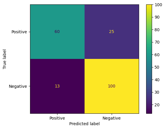
דרך מעניינת נוספת להערכת התחזיות של המודל היא מטריצות בלבול. מטריצת בלבול תציג באופן חזותי את הסוגים השונים של שגיאות חיזוי.

from sklearn.metrics import confusion_matrix, ConfusionMatrixDisplay

cm = confusion_matrix(y_true, y_pred)
ConfusionMatrixDisplay(
    confusion_matrix=cm,
    display_labels=agile_classifier.labels,
).plot()

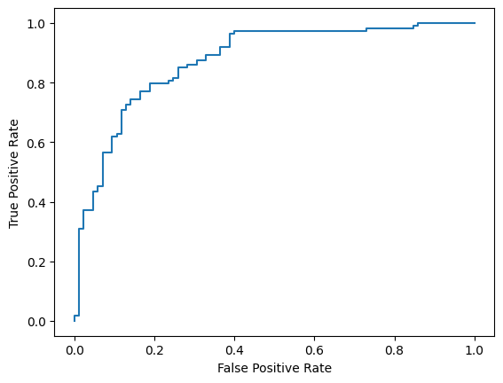
לבסוף, אפשר גם לעיין בעקומת ה-ROC כדי לקבל מושג לגבי שגיאות אפשריות בתחזיות כשמשתמשים בספי הערכה שונים.

from sklearn.metrics import RocCurveDisplay, roc_curve

fpr, tpr, _ = roc_curve(y_true, y_prob, pos_label=1)
RocCurveDisplay(fpr=fpr, tpr=tpr).plot()