1. 개요
이 Codelab에서는 파라미터 효율적인 튜닝 (PET)을 사용하여 맞춤 텍스트 분류기를 만드는 방법을 보여줍니다. PET 방법은 전체 모델을 미세 조정하는 대신 소량의 매개변수만 업데이트하므로 학습이 비교적 쉽고 빠릅니다. 또한 모델이 비교적 적은 학습 데이터로 새로운 동작을 더 쉽게 학습할 수 있습니다. 이 방법론은 모두를 위한 애자일 텍스트 분류기에 자세히 설명되어 있으며, 이 기법을 다양한 안전 작업에 적용하고 수백 개의 학습 예시만으로 최첨단 성능을 달성하는 방법을 보여줍니다.
이 Codelab에서는 더 빠르고 효율적으로 실행할 수 있으므로 LoRA PET 방법과 더 작은 Gemma 모델 (gemma_instruct_2b_en)을 사용합니다. 이 Colab에서는 데이터를 수집하고, LLM에 맞게 형식을 지정하고, LoRA 가중치를 학습시킨 다음 결과를 평가하는 단계를 다룹니다. 이 Codelab에서는 YouTube 및 Reddit 댓글로 구성된 증오심 표현 감지를 위한 공개 데이터 세트인 ETHOS 데이터 세트를 학습합니다. 데이터 세트의 1/4인 200개의 예시로만 학습한 경우 F1: 0.80, ROC-AUC: 0.78을 달성하여 리더보드에 현재 보고된 SOTA보다 약간 높습니다(2024년 2월 15일 작성 시점). 800개의 전체 예시로 학습하면 F1 점수 83.74, ROC-AUC 점수 88.17을 달성합니다. gemma_instruct_7b_en와 같은 대형 모델은 일반적으로 성능이 더 우수하지만 학습 및 실행 비용도 더 많이 듭니다.
트리거 경고: 이 Codelab에서는 증오심 표현을 감지하는 안전 분류기를 개발하므로 결과의 예시와 평가에는 일부 끔찍한 언어가 포함되어 있습니다.
2. 설치 및 설정
이 Codelab에서는 최신 버전의 keras (3), keras-nlp (0.8.0)이 필요하며 기본 모델을 다운로드할 Kaggle 계정이 필요합니다.
!pip install -q -U keras-nlp
!pip install -q -U keras
Kaggle에 로그인하려면 kaggle.json 사용자 인증 정보 파일을 ~/.kaggle/kaggle.json에 저장하거나 Colab 환경에서 다음을 실행하면 됩니다.
import kagglehub

kagglehub.login()
이 Codelab은 Keras 백엔드로 TensorFlow를 사용하여 테스트했지만 TensorFlow, Pytorch 또는 JAX를 사용할 수 있습니다.
import os

os.environ["KERAS_BACKEND"] = "tensorflow"
3. ETHOS 데이터 세트 로드
이 섹션에서는 분류기를 학습시킬 데이터 세트를 로드하고 학습 세트와 테스트 세트로 전처리합니다. 소셜 미디어에서 증오심 표현을 감지하기 위해 수집된 인기 있는 연구 데이터 세트인 ETHOS를 사용합니다. 데이터 세트가 수집된 방식에 관한 자세한 내용은 ETHOS: an Online Hate Speech Detection Dataset 논문을 참고하세요.
import pandas as pd

gh_root = 'https://raw.githubusercontent.com'
gh_repo = 'intelligence-csd-auth-gr/Ethos-Hate-Speech-Dataset'
gh_path = 'master/ethos/ethos_data/Ethos_Dataset_Binary.csv'
data_url = f'{gh_root}/{gh_repo}/{gh_path}'

df = pd.read_csv(data_url, delimiter=';')
df['hateful'] = (df['isHate'] >= df['isHate'].median()).astype(int)

# Shuffle the dataset.
df = df.sample(frac=1, random_state=32)

# Split into train and test.
df_train, df_test = df[:800],  df[800:]

# Display a sample of the data.
df.head(5)[['hateful', 'comment']]
다음과 비슷한 내용이 표시됩니다.
라벨 | 댓글 수 | |
0 |
|
|
1 |
|
|
2 |
|
|
3 |
|
|
4 |
|
|
4. 모델 다운로드 및 인스턴스화
문서에 설명된 대로 다양한 방식으로 Gemma 모델을 쉽게 사용할 수 있습니다. Keras를 사용하는 경우 다음을 실행해야 합니다.
import keras
import keras_nlp

# For reproducibility purposes.
keras.utils.set_random_seed(1234)

# Download the model from Kaggle using Keras.
model = keras_nlp.models.GemmaCausalLM.from_preset('gemma_instruct_2b_en')

# Set the sequence length to a small enough value to fit in memory in Colab.
model.preprocessor.sequence_length = 128
텍스트를 생성하여 모델이 작동하는지 테스트할 수 있습니다.
model.generate('Question: what is the capital of France? ', max_length=32)
5. 텍스트 전처리 및 구분자 토큰
모델이 의도를 더 잘 이해할 수 있도록 텍스트를 전처리하고 구분자 토큰을 사용할 수 있습니다. 이렇게 하면 모델이 예상 형식에 맞지 않는 텍스트를 생성할 가능성이 줄어듭니다. 예를 들어 다음과 같은 프롬프트를 작성하여 모델에 감정 분류를 요청할 수 있습니다.
Classify the following text into one of the following classes:[Positive,Negative]

Text: you look very nice today
Classification:
이 경우 모델이 원하는 내용을 출력할 수도 있고 출력하지 않을 수도 있습니다. 예를 들어 텍스트에 줄바꿈 문자가 포함되어 있으면 모델 성능에 부정적인 영향을 미칠 수 있습니다. 더 강력한 접근 방식은 구분자 토큰을 사용하는 것입니다. 그러면 프롬프트는 다음과 같이 됩니다.
Classify the following text into one of the following classes:[Positive,Negative]
<separator>
Text: you look very nice today
<separator>
Prediction:
텍스트를 전처리하는 함수를 사용하여 이를 추상화할 수 있습니다.
def preprocess_text(
    text: str,
    labels: list[str],
    instructions: str,
    separator: str,
) -> str:
  prompt = f'{instructions}:[{",".join(labels)}]'
  return separator.join([prompt, f'Text:{text}', 'Prediction:'])
이제 이전과 동일한 프롬프트와 텍스트를 사용하여 함수를 실행하면 동일한 출력이 표시됩니다.
text = 'you look very nice today'

prompt = preprocess_text(
    text=text,
    labels=['Positive', 'Negative'],
    instructions='Classify the following text into one of the following classes',
    separator='\n<separator>\n',
)

print(prompt)
다음과 같이 출력됩니다.
Classify the following text into one of the following classes:[Positive,Negative]
<separator>
Text:well, looks like its time to have another child
<separator>
Prediction:
6. 출력 후처리
모델의 출력은 다양한 확률을 갖는 토큰입니다. 일반적으로 텍스트를 생성하려면 가능성이 가장 높은 상위 몇 개의 토큰 중에서 선택하고 문장, 단락 또는 전체 문서를 구성합니다. 하지만 분류의 목적에서는 모델이 Positive이 Negative보다 더 가능성이 높다고 생각하는지 아니면 그 반대인지가 실제로 중요합니다.
앞서 인스턴스화한 모델이 주어지면 다음 토큰이 Positive인지 Negative인지에 대한 독립적인 확률로 출력을 처리하는 방법은 다음과 같습니다.
import numpy as np


def compute_output_probability(
    model: keras_nlp.models.GemmaCausalLM,
    prompt: str,
    target_classes: list[str],
) -> dict[str, float]:
  # Shorthands.
  preprocessor = model.preprocessor
  tokenizer = preprocessor.tokenizer

  # NOTE: If a token is not found, it will be considered same as "<unk>".
  token_unk = tokenizer.token_to_id('<unk>')

  # Identify the token indices, which is the same as the ID for this tokenizer.
  token_ids = [tokenizer.token_to_id(word) for word in target_classes]

  # Throw an error if one of the classes maps to a token outside the vocabulary.
  if any(token_id == token_unk for token_id in token_ids):
    raise ValueError('One of the target classes is not in the vocabulary.')

  # Preprocess the prompt in a single batch. This is done one sample at a time
  # for illustration purposes, but it would be more efficient to batch prompts.
  preprocessed = model.preprocessor.generate_preprocess([prompt])

  # Identify output token offset.
  padding_mask = preprocessed["padding_mask"]
  token_offset = keras.ops.sum(padding_mask) - 1

  # Score outputs, extract only the next token's logits.
  vocab_logits = model.score(
      token_ids=preprocessed["token_ids"],
      padding_mask=padding_mask,
  )[0][token_offset]

  # Compute the relative probability of each of the requested tokens.
  token_logits = [vocab_logits[ix] for ix in token_ids]
  logits_tensor = keras.ops.convert_to_tensor(token_logits)
  probabilities = keras.activations.softmax(logits_tensor)

  return dict(zip(target_classes, probabilities.numpy()))
앞서 만든 프롬프트로 함수를 실행하여 테스트할 수 있습니다.
compute_output_probability(
    model=model,
    prompt=prompt,
    target_classes=['Positive', 'Negative'],
)
그러면 다음과 비슷한 결과가 출력됩니다.
{'Positive': 0.99994016, 'Negative': 5.984089e-05}
7. 모두 분류기로 래핑
사용 편의성을 위해 방금 만든 모든 함수를 predict(), predict_score()과 같이 사용하기 쉽고 친숙한 함수가 있는 단일 sklearn과 유사한 분류기로 래핑할 수 있습니다.
import dataclasses


@dataclasses.dataclass(frozen=True)
class AgileClassifier:
  """Agile classifier to be wrapped around a LLM."""

  # The classes whose probability will be predicted.
  labels: tuple[str, ...]

  # Provide default instructions and control tokens, can be overridden by user.
  instructions: str = 'Classify the following text into one of the following classes'
  separator_token: str = '<separator>'
  end_of_text_token: str = '<eos>'

  def encode_for_prediction(self, x_text: str) -> str:
    return preprocess_text(
        text=x_text,
        labels=self.labels,
        instructions=self.instructions,
        separator=self.separator_token,
    )

  def encode_for_training(self, x_text: str, y: int) -> str:
    return ''.join([
        self.encode_for_prediction(x_text),
        self.labels[y],
        self.end_of_text_token,
    ])

  def predict_score(
      self,
      model: keras_nlp.models.GemmaCausalLM,
      x_text: str,
  ) -> list[float]:
    prompt = self.encode_for_prediction(x_text)
    token_probabilities = compute_output_probability(
        model=model,
        prompt=prompt,
        target_classes=self.labels,
    )
    return [token_probabilities[token] for token in self.labels]

  def predict(
      self,
      model: keras_nlp.models.GemmaCausalLM,
      x_eval: str,
  ) -> int:
    return np.argmax(self.predict_score(model, x_eval))


agile_classifier = AgileClassifier(labels=('Positive', 'Negative'))
8. 모델 미세 조정
LoRA는 Low-Rank Adaptation의 약자입니다. 대규모 언어 모델을 효율적으로 미세 조정하는 데 사용할 수 있는 미세 조정 기법입니다. 자세한 내용은 LoRA: 대규모 언어 모델의 하위 순위 조정 논문을 참고하세요.
Gemma의 Keras 구현은 미세 조정에 사용할 수 있는 enable_lora() 메서드를 제공합니다.
# Enable LoRA for the model and set the LoRA rank to 4.
model.backbone.enable_lora(rank=4)
LoRA를 사용 설정한 후 미세 조정 프로세스를 시작할 수 있습니다. Colab에서 에포크당 약 5분이 걸립니다.
import tensorflow as tf

# Create dataset with preprocessed text + labels.
map_fn = lambda xy: agile_classifier.encode_for_training(*xy)
x_train = list(map(map_fn, df_train[['comment', 'hateful']].values))
ds_train = tf.data.Dataset.from_tensor_slices(x_train).batch(2)

# Compile the model using the Adam optimizer and appropriate loss function.
model.compile(
    loss=keras.losses.SparseCategoricalCrossentropy(from_logits=True),
    optimizer=keras.optimizers.Adam(learning_rate=0.0005),
    weighted_metrics=[keras.metrics.SparseCategoricalAccuracy()],
)

# Begin training.
model.fit(ds_train, epochs=4)
과적합이 발생할 때까지 더 많은 에포크로 학습하면 정확도가 높아집니다.
9. 결과 검사
이제 방금 학습한 애자일 분류기의 출력을 검사할 수 있습니다. 이 코드는 텍스트가 주어지면 예측된 클래스 점수를 출력합니다.
text = 'you look really nice today'
scores = agile_classifier.predict_score(model, text)
dict(zip(agile_classifier.labels, scores))
{'Positive': 0.99899644, 'Negative': 0.0010035498}
10. 모델 평가
마지막으로 F1 점수와 AUC-ROC라는 두 가지 일반적인 측정항목을 사용하여 모델의 성능을 평가합니다. F1 점수는 특정 분류 기준점에서 정밀도와 재현율의 조화 평균을 평가하여 거짓음성 및 거짓양성 오류를 포착합니다. 반면 AUC-ROC는 다양한 임곗값에서 참양성률과 거짓양성률 간의 균형을 포착하고 이 곡선 아래의 면적을 계산합니다.
from sklearn.metrics import f1_score, roc_auc_score

y_true = df_test['hateful'].values
# Compute the scores (aka probabilities) for each of the labels.
y_score = [agile_classifier.predict_score(model, x) for x in df_test['comment']]
# The label with highest score is considered the predicted class.
y_pred = np.argmax(y_score, axis=1)
# Extract the probability of a comment being considered hateful.
y_prob = [x[agile_classifier.labels.index('Negative')] for x in y_score]

# Compute F1 and AUC-ROC scores.
print(f'F1: {f1_score(y_true, y_pred):.2f}')
print(f'AUC-ROC: {roc_auc_score(y_true, y_prob):.2f}')
F1: 0.84
AUC-ROC: = 0.88
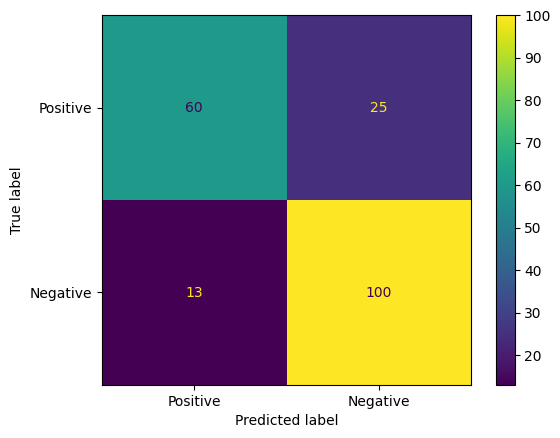
모델 예측을 평가하는 또 다른 흥미로운 방법은 혼동 행렬입니다. 혼동 행렬은 다양한 종류의 예측 오류를 시각적으로 보여줍니다.
from sklearn.metrics import confusion_matrix, ConfusionMatrixDisplay

cm = confusion_matrix(y_true, y_pred)
ConfusionMatrixDisplay(
    confusion_matrix=cm,
    display_labels=agile_classifier.labels,
).plot()
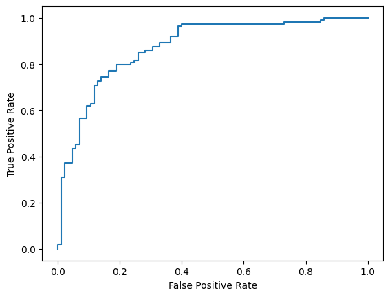
마지막으로 ROC 곡선을 살펴보고 다양한 점수 임곗값을 사용할 때 발생할 수 있는 예측 오류를 파악할 수도 있습니다.
from sklearn.metrics import RocCurveDisplay, roc_curve

fpr, tpr, _ = roc_curve(y_true, y_prob, pos_label=1)
RocCurveDisplay(fpr=fpr, tpr=tpr).plot()