
1. Introduction
In this codelab, you will learn how to leverage BigQuery Graph to solve complex supply chain and logistics problems.
You will model a restaurant supply chain network focusing on food safety and quality control. When a food safety issue arises—such as a contaminated ingredient from a supplier—time is of the essence. Identifying the "blast radius" and executing a surgical recall quickly can save costs and protect customers.

Traditional relational models require complex, multi-step JOIN operations to trace items through multiple stages (Supplier -> DC -> Commissary -> Store -> Finished Item). With BigQuery Graph, we model these connections directly, enabling intuitive and fast queries using the ISO GQL (Graph Query Language) standard.
What you'll learn
- How to define a graph model on top of existing BigQuery tables.
- How to create a Property Graph inside BigQuery.
- How to run traversal queries to trace upstream and downstream impacts.
What you'll need
- A Google Cloud Project with billing enabled.
- Google Cloud Shell.
Cost Estimate
This lab is expected to cost less than $5 USD in BigQuery analysis fees, well within the Free Tier allocations for new users.
2. Setup and Requirements
Open Cloud Shell
You will perform the majority of the work in Cloud Shell, a loaded environment that rolls with everything you need to use Google Cloud.
- Go to the Google Cloud Console.
- Click the Activate Cloud Shell icon in the top right toolbar.
- Click Continue if prompted.
Set up Environment Variables
In Cloud Shell, set your Project ID to simplify future commands.
export PROJECT_ID=$(gcloud config get-value project)
Enable BigQuery API
Ensure the BigQuery API is enabled. It is usually enabled by default, but it is best to be safe.
gcloud services enable bigquery.googleapis.com
3. Creating the Schema and Tables
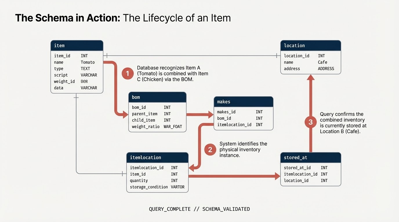
You will create a dataset and tables representing your supply chain components:
item: The generic item definition (e.g., Tomato, Chicken).location: Facilities (Suppliers, distribution centers, cafes).itemlocation: The intersection table representing inventory locations.bom: Bill of Materials (defines weight relations, e.g. Item A goes into Item B).makes: Mapsitemlocationto theitem.stored_at: Mapsitemlocationtolocation.
Create Dataset
You can run the SQL commands in this lab using either Cloud Shell or the BigQuery Console.
To use the BigQuery console:
- Open the BigQuery Console in a new tab.
- Paste each SQL snippet from this lab into the editor, then click the Run button to execute it.
Run the following command in Cloud Shell or use the BigQuery Console to create the schema. You will use node variables in your SQL.
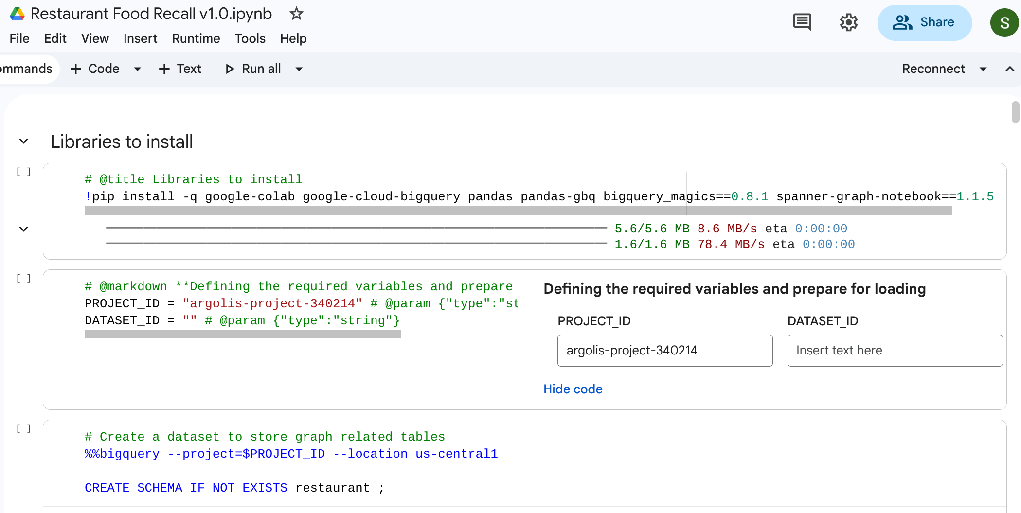
Note: (1) To execute this in Google Colab, you can also use the BigQuery magic commands: %%bigquery The following snippet creates the restaurant schema within your project to house your graph data. (2) You will need to use %%bigquery –project <PROJECT_ID> if you are running from a Google Colab. Make sure the field PROJECT_ID is mapped to the appropriate project you intend to use: PROJECT_ID = "argolis-project-340214" # @param {"type":"string"} (3) If you are using colab, then depending upon your requirements you will need to install some libraries. If you are going to be using graph visualization make sure you pip install the library: spanner-graph-notebook==1.1.5
%%bigquery --project=$PROJECT_ID
CREATE SCHEMA IF NOT EXISTS restaurant ;
Create Tables
Execute the following SQL code to build the tables.
%%bigquery --project=$PROJECT_ID
-- 1. Item Table
DROP TABLE IF EXISTS `restaurant.item`;
CREATE TABLE `restaurant.item` (
  itemKey STRING,
  itemName STRING,
  itemCategory STRING,
  shelfLifeDays INT64,
  PRIMARY KEY (itemKey) NOT ENFORCED
);

-- 2. Location Table
DROP TABLE IF EXISTS `restaurant.location`;
CREATE TABLE `restaurant.location` (
  locationKey STRING,
  locationType STRING,
  locationCity STRING,
  locationState STRING,
  dunsNumber INT64,
  PRIMARY KEY (locationKey) NOT ENFORCED
);
-- 3. ItemLocation Table
DROP TABLE IF EXISTS `restaurant.itemlocation`;
CREATE TABLE `restaurant.itemlocation` (
  itemLocationKey STRING,
  itemKey STRING,
  locationKey STRING,
  variants INT64,
  PRIMARY KEY (itemLocationKey) NOT ENFORCED,
  -- Foreign Key Definitions
  FOREIGN KEY (itemKey) REFERENCES `restaurant.item`(itemKey) NOT ENFORCED,
  FOREIGN KEY (locationKey) REFERENCES `restaurant.location`(locationKey) NOT ENFORCED
);

-- 4. BOM Table
DROP TABLE IF EXISTS `restaurant.bom`;
CREATE TABLE `restaurant.bom` (
  bomKey INT64,
  parentItemLocation STRING,
  childItemLocation STRING,
  childQuantity FLOAT64,
  PRIMARY KEY (bomKey) NOT ENFORCED
);

-- 5. Makes Table
DROP TABLE IF EXISTS `restaurant.makes`;
CREATE TABLE `restaurant.makes` (
  itemLocationKey STRING,
  itemKey STRING,
  locationKey STRING,
  variants INT64,
  PRIMARY KEY (itemLocationKey) NOT ENFORCED
);

DROP TABLE IF EXISTS `restaurant.stored_at`;
CREATE TABLE `restaurant.stored_at` (
  itemLocationKey STRING,
  itemKey STRING,
  locationKey STRING,
  variants INT64,
  PRIMARY KEY (itemLocationKey) NOT ENFORCED
);
4. Loading Sample Data
To make this lab fully self-contained, you will populate the tables with sample data using pure SQL LOAD DATA statements. This represents a network starting with a Supplier, traversing through a Distribution Center (DC) and Commissary Kitchen, and landing at a Retail Café.
Run the following SQL queries to load the data:

Note: You can omit %%bigquery if you are running directly in bigquery studio
%%bigquery --project=$PROJECT_ID
-- Load Item
LOAD DATA OVERWRITE `restaurant.item`
FROM FILES (format = 'CSV', uris = ['gs://supply_chain_demo/item2.csv'], skip_leading_rows = 1);

-- Load Location
LOAD DATA OVERWRITE `restaurant.location`
FROM FILES (format = 'CSV', uris = ['gs://supply_chain_demo/location.csv'], skip_leading_rows = 1);

-- Load ItemLocation
LOAD DATA OVERWRITE `restaurant.itemlocation`
FROM FILES (format = 'CSV', uris = ['gs://supply_chain_demo/itemlocation.csv'], skip_leading_rows = 1);

-- Load BOM
LOAD DATA OVERWRITE `restaurant.bom`
FROM FILES (format = 'CSV', uris = ['gs://supply_chain_demo/bom2.csv'], skip_leading_rows = 1);

-- Load Makes
LOAD DATA OVERWRITE `restaurant.makes`
FROM FILES (format = 'CSV', uris = ['gs://supply_chain_demo/makes.csv'], skip_leading_rows = 1);

-- Load StoredAt
LOAD DATA OVERWRITE `restaurant.stored_at`
FROM FILES (format = 'CSV', uris = ['gs://supply_chain_demo/itemlocation.csv'], skip_leading_rows = 1);
5. Adding Constraints and Defining Graph
Before building the graph, you declare the semantic relationships using standard SQL Primary Key and Foreign Key constraints. These guide BigQuery in understanding Node identifiers and connecting Edge tables to Node tables.
Create Property Graph
Now, you unite these tables into a single cohesive Graph structure called restaurant.bombod.
You define:
- Nodes:
item,location,itemlocation - Edges:
makes,stored_at, andconsists_of(BOM)
%%bigquery --project=$PROJECT_ID

CREATE OR REPLACE PROPERTY GRAPH `restaurant.bombod`
NODE TABLES (
  `restaurant.item` KEY (itemKey) LABEL item PROPERTIES ALL COLUMNS,
  `restaurant.location` KEY (locationKey) LABEL location PROPERTIES ALL COLUMNS,
  `restaurant.itemlocation` KEY (itemLocationKey) LABEL itemlocation PROPERTIES ALL COLUMNS
)
EDGE TABLES (
  `restaurant.makes`
    KEY (itemLocationKey)
    SOURCE KEY (itemLocationKey) REFERENCES `restaurant.itemlocation`(itemLocationKey)
    DESTINATION KEY (itemKey) REFERENCES `restaurant.item`(itemKey)
    LABEL makes PROPERTIES ALL COLUMNS,

  `restaurant.bom`
    KEY (bomKey)
    SOURCE KEY (childItemLocation) REFERENCES `restaurant.itemlocation`(itemLocationKey)
    DESTINATION KEY (parentItemLocation) REFERENCES `restaurant.itemlocation`(itemLocationKey)
    LABEL consists_of PROPERTIES ALL COLUMNS,

  `restaurant.stored_at`
    KEY (itemLocationKey)
    SOURCE KEY (itemLocationKey) REFERENCES `restaurant.itemlocation`(itemLocationKey)
    DESTINATION KEY (locationKey) REFERENCES `restaurant.location`(locationKey)
    LABEL stored_at PROPERTIES ALL COLUMNS
);
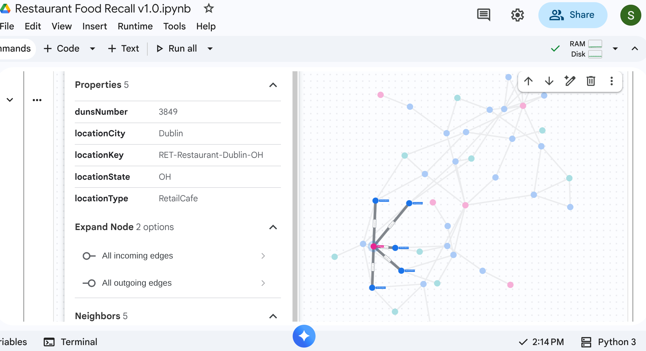
6. Visualizing the Supply Chain
You can run a top-down traversal query to see the entire supply chain network. In a standard notebook or UI that supports it (such as %%bigquery --graph), this returns a visual map.
Use absolute graph queries to get nodes and edges setup.
Note: As mentioned earlier, to execute this in Google Colab or Colab Enterprise Notebooks, you can also use the BigQuery magic commands: %%bigquery Also to visualize the graph in Google Colab or Colab Enterprise Notebooks include the –graph flag as: %%bigquery –graph
%%bigquery  --project=$PROJECT_ID --graph output

Graph restaurant.bombod

match p=(a:itemlocation)-[c:consists_of]->(b:itemlocation)
match q=(a)-[d:stored_at]->(e:location)
optional match z=(f)-[g:makes]-(b)

return to_json(p) as ppath, to_json(q) as qpath, to_json(z) as zpath
Output:
7. Use Case 1: Tracing an Upstream Complaint
Scenario: A customer complains about the quality of the chicken in their sandwich at the New York store. You need to trace the finished item backward to see its immediate assembly stages.
Traversal Query
Run the query using the Graph Traversal query format. This looks at the consists_of edges that relate assemblies downstream up to upstream ingredients.
%%bigquery --project=$PROJECT_ID --graph

GRAPH restaurant.bombod
MATCH p=(a:itemlocation)-[c:consists_of]->(b:itemlocation)
OPTIONAL MATCH q=(b)-[d:stored_at]-(e)
return to_json(p) as ppath, to_json(q) as qpath
Because of the arrow direction in the consists_of Edge Table (Ingredient -> Finished), a search flowing upstream yields links quickly isolating dependent materials and storage locations.
Output: 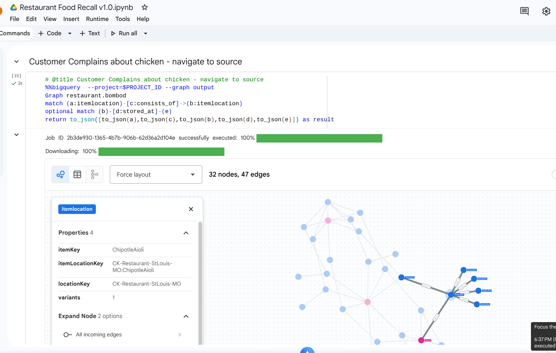
8. Use Case 2: Impact Analysis
Scenario: A snowstorm has shut down the Distribution Center in Columbus, OH. You need to know which downstream preparations or finished items are immediately affected.
Traversal Query
You start at the specific location representing the Distribution Center, identify the inventory stored there, and see what finished items require them.
# @title Impact of a storm on a DC

%%bigquery  --project=$PROJECT_ID --graph
Graph restaurant.bombod
match path1=(z:itemlocation)-[m:stored_at]->(dc:location) where dc.locationKey like '%DC-Sysco-Columbus-OH%'
match path2=(z:itemlocation)-[c:consists_of]->(b:itemlocation)
match path3=(b:itemlocation)-[n:makes]->(item:item)
optional match path4=(b)-[p:stored_at]->(q:location)
return to_json(path1) as path1, to_json(path2) as path2,to_json(path3) as path3, to_json(path4) as path4
Output: 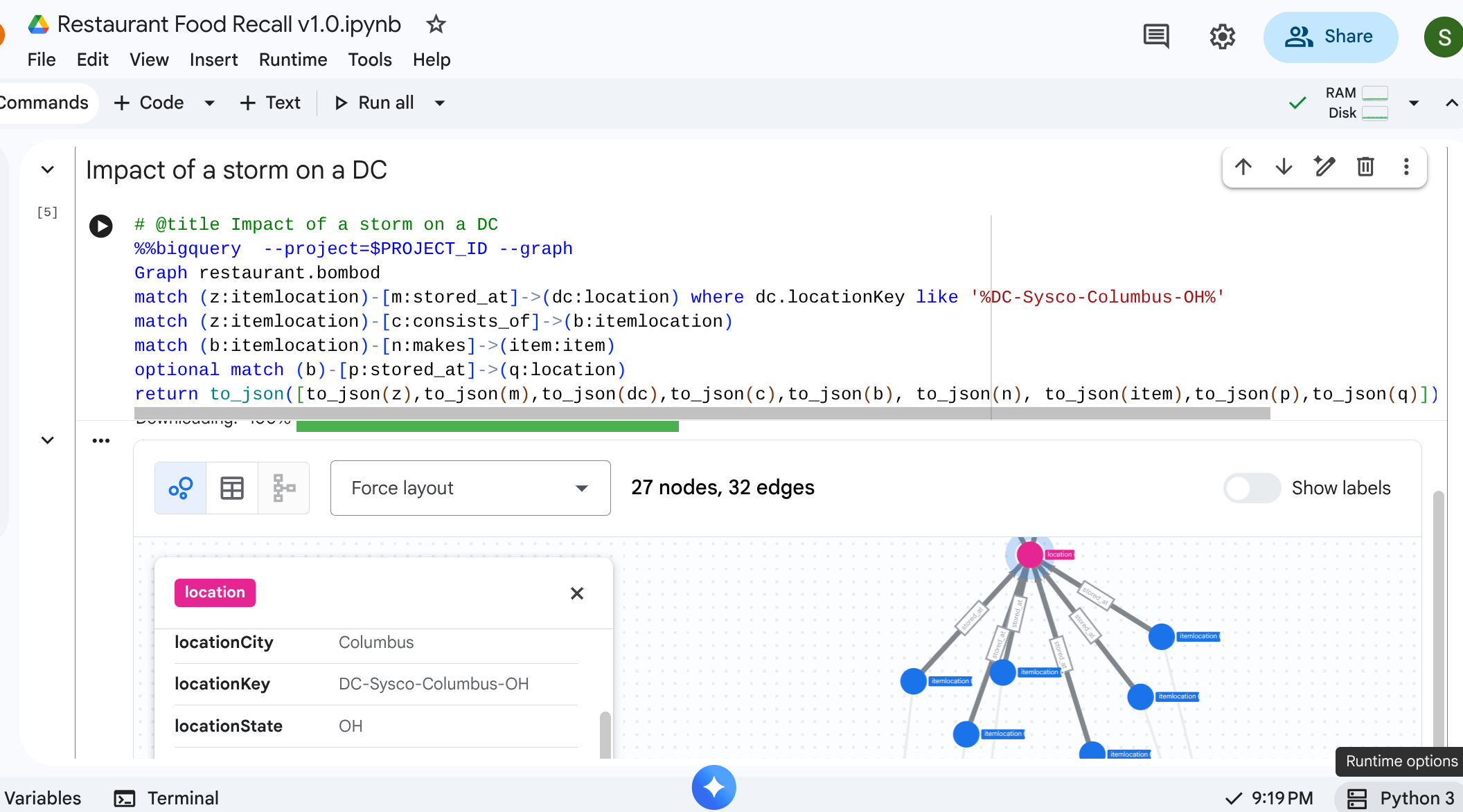
9. Use Case 3: Downstream Recall
Scenario: A supplier notifies you of a specific batch of contaminated product: Vine-Ripened Tomatoes from the Supplier. You need to find all affected final menu items at the cafes.
Traversal Query
You look for the contaminated raw material location, then perform a path traversal flowing downstream to find the ultimate impacted items.
%%bigquery  --project=$PROJECT_ID --graph
Graph restaurant.bombod
match path1=(a:itemlocation)-[c:consists_of]->(b:itemlocation)-[e:makes]->(f:item) where f.itemKey like '%Tomato%'
return to_json(path1) as result
This query locates all items that pattern match with ‘Tomato' and that is intertwined with the upstream relationship making it a powerful mapping that propagates to discover which cafe items must be recalled.
Output: 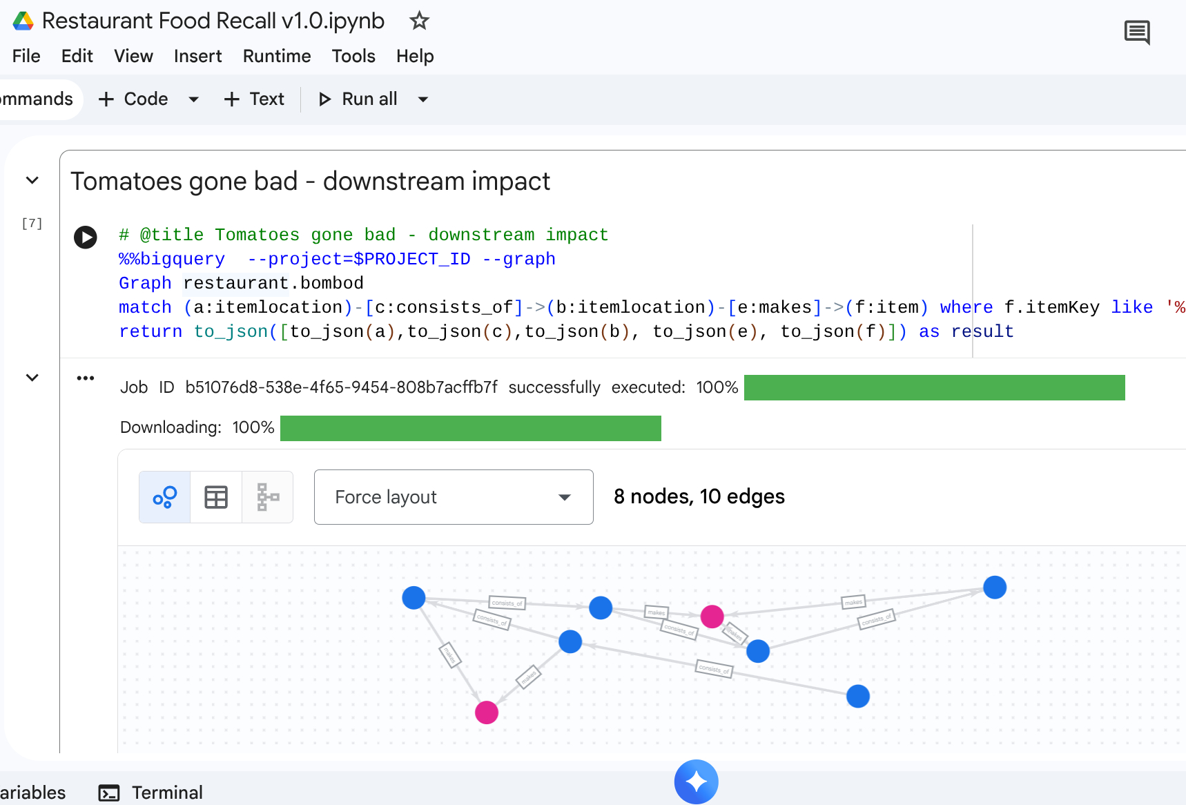
10. Clean Up
Delete resources once you complete the walkthrough steps to avoid any residual charges in your workspace.
DROP SCHEMA `restaurant` CASCADE;
11. Conclusion
Congratulations! You've modeled a supply chain and executed impact analysis using BigQuery Graph.
Wrap up
You learned to:
- Declare graph-centric relational relationships with Primary/Foreign keys.
- Create a Unified Property Graph.
- Navigate multi-node relationships efficiently using Graph Query traversal logic.
To gain more graph architecture insights, visit the Google Cloud docs.