מדעי הנתונים עם Spark

1. סקירה כללית

חברת TheLook, קמעונאית היפותטית של בגדים למסחר אלקטרוני, מאחסנת נתונים על לקוחות, מוצרים, הזמנות, לוגיסטיקה, אירועים באתר וקמפיינים של שיווק דיגיטלי ב-BigQuery. החברה רוצה להשתמש במומחיות הקיימת של הצוות ב-SQL וב-PySpark כדי לנתח את הנתונים האלה באמצעות Apache Spark.

כדי להימנע מהקצאה או מכוונון ידני של התשתית ל-Spark, חברת TheLook מחפשת פתרון של התאמה אוטומטית לעומס שיאפשר לה להתמקד בעומסי העבודה ולא בניהול האשכולות. בנוסף, הם רוצים לצמצם את המאמץ הנדרש לשילוב של Spark ו-BigQuery, תוך שמירה על סביבת BigQuery Studio.

בשיעור Lab הזה תבנו מסווג רגרסיה לוגיסטית באמצעות PySpark ותשתמשו בשילוב המובנה של מחברות ב-BigQuery Studio ובתכונות ה-AI כדי לחקור את הנתונים, במטרה לחזות אם משתמש יבצע רכישה. פורסים את המודל הזה בשרת הסקת מסקנות ויוצרים סוכן לשליחת שאילתות למודל בשפה טבעית.

דרישות מוקדמות

לפני שמתחילים את שיעור ה-Lab הזה, חשוב להכיר את הנושאים הבאים:

• תכנות בסיסי ב-SQL וב-Python.
• הרצת קוד Python ב-notebook של Jupyter.
• הבנה בסיסית של חישוב מבוזר

יעדים

• משתמשים במחברות BigQuery Studio כדי להריץ תהליך עבודה של מדעי הנתונים.
• יוצרים חיבור ל-Apache Spark באמצעות Google Cloud Serverless ל-Apache Spark ומופעל על ידי Spark Connect.
• אפשר להשתמש ב-Lightning Engine כדי להאיץ את עומסי העבודה של Apache Spark עד פי 4.3.
• טוענים נתונים מ-BigQuery באמצעות השילוב המובנה בין Apache Spark ל-BigQuery.
• לנתח את הנתונים באמצעות יצירת קוד בעזרת Gemini.
• ביצוע הנדסת פיצ'רים (feature engineering) באמצעות מסגרת עיבוד הנתונים של Apache Spark.
• אימון והערכה של מודל סיווג באמצעות ספריית למידת המכונה המקורית של Apache Spark, ‏ MLlib.
• פריסת שרת היקשים למודל הסיווג באמצעות Flask ו-Cloud Run
• פריסת סוכן לשליחת שאילתות לשרת ההסקות באמצעות שפה טבעית עם Agent Engine ו-Agent Development Kit (ערכה לפיתוח סוכנים, ADK).

2. התחברות לסביבת זמן ריצה ב-Colab

זיהוי פרויקט ב-Google Cloud

יוצרים פרויקט ב-Google Cloud. אפשר להשתמש באחד קיים.

מפעילים את ממשקי ה-API המומלצים:

לוחצים כאן כדי להפעיל את ממשקי ה-API הבאים:

• aiplatform.googleapis.com
• bigquery.googleapis.com
• bigquerystorage.googleapis.com
• bigqueryunified.googleapis.com
• cloudaicompanion.googleapis.com
• dataproc.googleapis.com
• storage.googleapis.com
• run.googleapis.com

ניווט בממשק המשתמש:

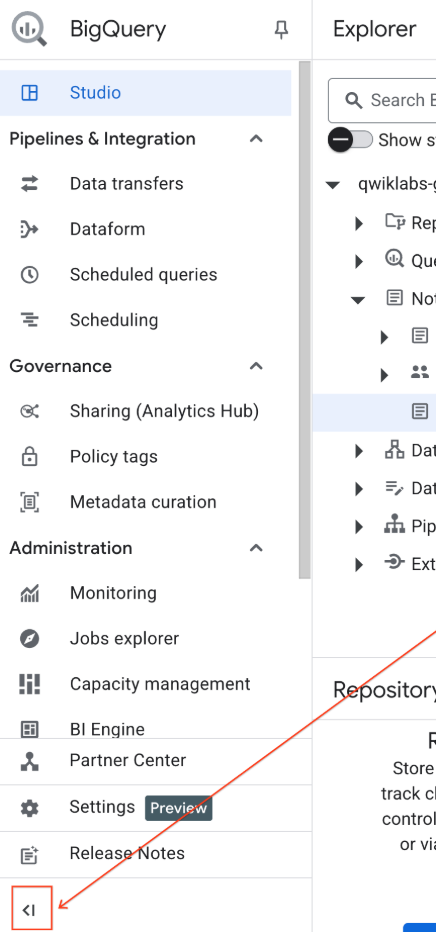
1. במסוף Google Cloud, עוברים אל תפריט הניווט > BigQuery.

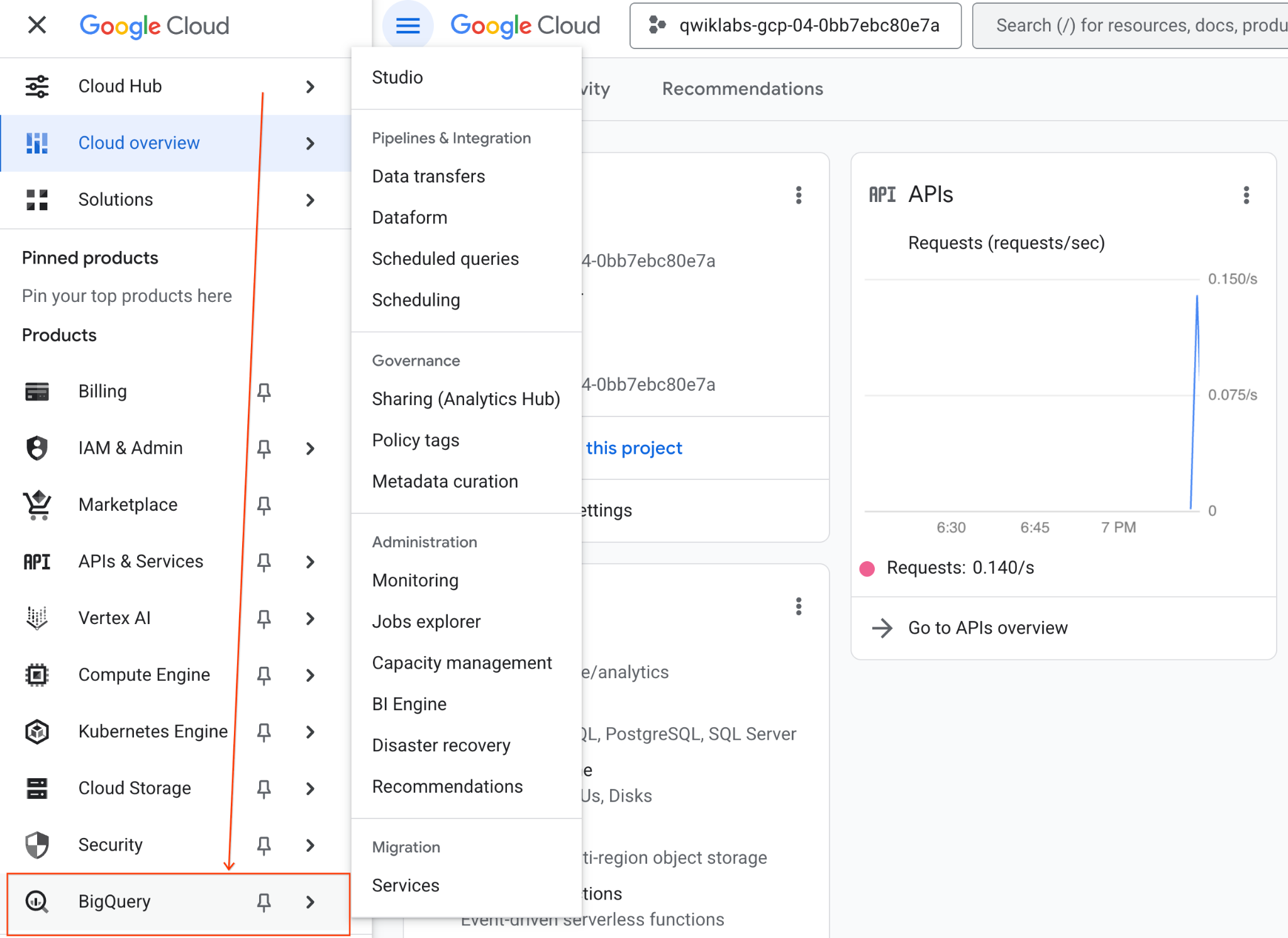
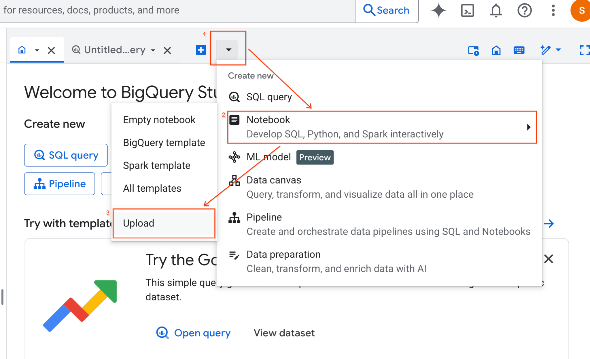
2. בחלונית BigQuery Studio, לוחצים על לחצן החץ של התפריט הנפתח, מעבירים את העכבר מעל Notebook ואז בוחרים באפשרות Upload (העלאה).

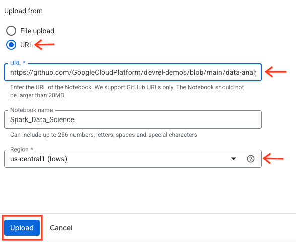
3. לוחצים על לחצן הבחירה של כתובת ה-URL ומזינים את כתובת ה-URL הבאה:

https://github.com/GoogleCloudPlatform/devrel-demos/blob/main/data-analytics/dataproc-webinar/data-science/Spark_Data_Science.ipynb

4. מגדירים את האזור ל-us-central11 ולוחצים על העלאה.

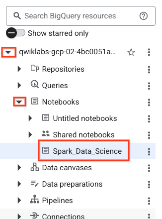
5. כדי לפתוח את ה-notebook, לוחצים על החץ לתפריט הנפתח בחלונית Explorer עם השם של מזהה הפרויקט. לוחצים על התפריט הנפתח מחברות. לוחצים על ה-Notebook Spark_Data_Science.

6. כדי לפנות מקום, אפשר לכווץ את תפריט הניווט של BigQuery ואת תוכן העניינים של המחברת.

3. התחברות לסביבת זמן ריצה והרצת קוד הגדרה נוסף

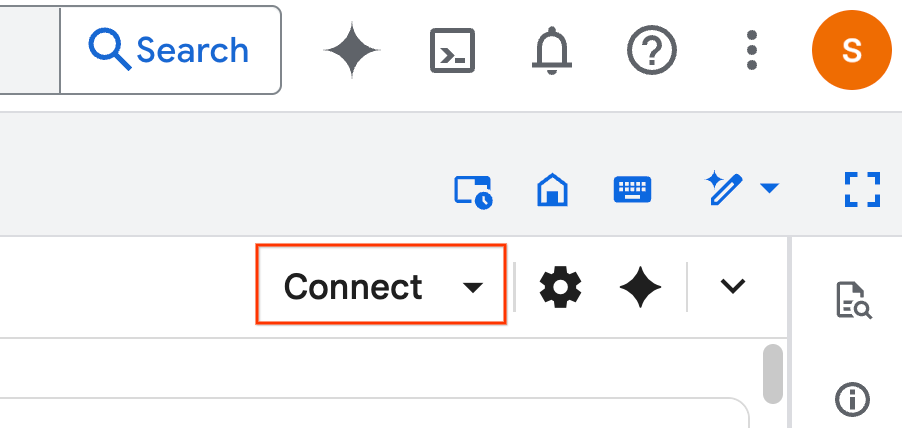
1. לוחצים על התחברות. בחלון הקופץ, מאשרים את Colab Enterprise באמצעות חשבון האימייל. ה-notebook יתחבר אוטומטית לסביבת ריצה.

הערה: יכול להיות שהפעולה תימשך כמה דקות.

2. אחרי שהסביבה תוגדר, תראו את הדברים הבאים:

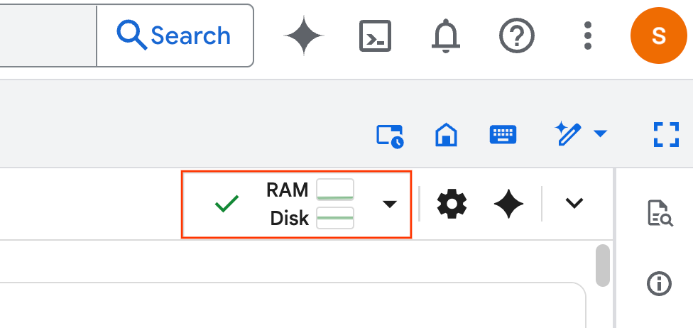
3. במחברת, גוללים לקטע הגדרה. מתחילים כאן.

הערה: אחרי שפותחים את קובץ ה-notebook, העבודה מתבצעת בעיקר בסביבת Colab. ה-notebook הזה מכיל את כל הקוד והסברים מפורטים, תא אחר תא, לכל תהליך העבודה. שיעור ה-Lab הזה הוא מדריך ברמה גבוהה, שכולל סיכומים קצרים שיעזרו לכם לעקוב אחרי ההתקדמות. אתם יכולים להפסיק לקרוא את ה-codelab כאן.

4. הרצת קוד ההגדרה

מגדירים את הסביבה עם ספריות Python הנדרשות כדי להשלים את ה-Lab. הגדרת גישה פרטית ל-Google. יוצרים קטגוריית אחסון. יוצרים מערך נתונים ב-BigQuery. מעתיקים את מזהה הפרויקט למחברת. בוחרים אזור. בשיעור ה-Lab הזה, משתמשים באזור us-central1.

כדי להריץ תא קוד, מעבירים את הסמן לתוך בלוק התא ולוחצים על החץ.

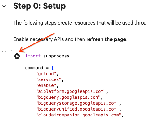
# Enable APIs
import subprocess

command = [
    "gcloud",
    "services",
    "enable",
    "aiplatform.googleapis.com",
    "bigquery.googleapis.com",
    "bigquerystorage.googleapis.com",
    "bigqueryunified.googleapis.com",
    "cloudaicompanion.googleapis.com",
    "dataproc.googleapis.com",
    "run.googleapis.com",
    "storage.googleapis.com"
]

result = subprocess.run(command, capture_output=True, text=True)
print(result.stdout)
print(result.stderr)

# Configure a PROJECT_ID and REGION
PROJECT_ID = "<YOUR_PROJECT_ID>"
REGION = "<YOUR_REGION>"

# Enable Private Google Access
import subprocess

command = [
    "gcloud",
    "compute",
    "networks",
    "subnets",
    "update",
    "default",
    f"--region={REGION}",
    "--enable-private-ip-google-access"
]

result = subprocess.run(command, capture_output=True, text=True)
print(result.stdout)
print(result.stderr)

# Create a Cloud Storage Bucket
from google.cloud import storage
from google.cloud.exceptions import NotFound

BUCKET_NAME = f"{PROJECT_ID}-demo"

storage_client = storage.Client(project=PROJECT_ID)
try:
    bucket = storage_client.get_bucket(BUCKET_NAME)
    print(f"Bucket {BUCKET_NAME} already exists.")
except NotFound:
    bucket = storage_client.create_bucket(BUCKET_NAME, location=REGION)
    print(f"Bucket {BUCKET_NAME} created.")


# Create a BigQuery dataset.
from google.cloud import bigquery

DATASET_ID = f"{PROJECT_ID}.demo"

client = bigquery.Client()

dataset = bigquery.Dataset(DATASET_ID)

dataset.location = REGION

dataset = client.create_dataset(dataset, exists_ok=True)

5. יצירת חיבור ל-Google Cloud Serverless ל-Apache Spark

באמצעות Spark Connect, אתם מתחברים לסשן Spark ללא שרת כדי להפעיל משימות אינטראקטיביות של Spark. אתם מגדירים את זמן הריצה באמצעות Lightning Engine לביצועים מתקדמים של Spark. ‫Lightning Engine פועל על ידי האצת עומסי עבודה באמצעות Apache Gluten ו-Velox.

from google.cloud.dataproc_spark_connect import DataprocSparkSession
from google.cloud.dataproc_v1 import Session

session = Session()

session.runtime_config.version = "3.0"

# You can optionally configure Spark properties as well. See https://cloud.google.com/dataproc-serverless/docs/concepts/properties.
session.runtime_config.properties = {
  "dataproc.runtime": "premium",
  "spark.dataproc.engine": "lightningEngine",
}

# To avoid going over quota in this demo, cap the max number of Spark workers.
session.runtime_config.properties = {
    "spark.dynamicAllocation.maxExecutors": "4"
}

spark = (
    DataprocSparkSession.builder
      .appName("CustomSparkSession")
      .dataprocSessionConfig(session)
      .getOrCreate()
)

6. טעינה של נתונים וחקירה שלהם באמצעות Gemini

בקטע הזה תעברו על השלב החשוב הראשון בכל פרויקט של מדעי הנתונים: הכנת הנתונים. מתחילים בטעינת נתונים לתוך מסגרת נתונים של Apache Spark מ-BigQuery.

# Load the tables
order_items = spark.read.format("bigquery").option("table", "bigquery-public-data.thelook_ecommerce.order_items").load()

users = spark.read.format("bigquery").option("table", "bigquery-public-data.thelook_ecommerce.users").load()

# Register temp tables
users.createOrReplaceTempView("users")
order_items.createOrReplaceTempView("order_items")

# Verify temp tables
spark.sql("SELECT * FROM order_items LIMIT 10").show()

לאחר מכן, אתם משתמשים ב-Gemini כדי ליצור קוד PySpark כדי לחקור את הנתונים ולהבין אותם טוב יותר.

הנחיה 1: באמצעות PySpark, בודקים את טבלת המשתמשים ומציגים את 10 השורות הראשונות.

# prompt:  Using PySpark, explore the users table and show the first 10 rows.

users.show(10)

הנחיה 2: באמצעות PySpark, בודקים את הטבלה order_items ומציגים את 10 השורות הראשונות.

# prompt: Using PySpark, explore the order_items table and show the first 10 rows.

order_items.show(10)

הנחיה 3: באמצעות PySpark, הצג את 5 המדינות הנפוצות ביותר בטבלת המשתמשים. הצגת המדינה ומספר המשתמשים מכל מדינה.

# prompt: Using PySpark, show the top 5 most frequent countries in the users table. Display the country and the number of users from each country.

from pyspark.sql.functions import col, count

users.groupBy("country").agg(count("*").alias("user_count")).orderBy(col("user_count").desc()).limit(5).show()

הנחיה 4: באמצעות PySpark, צריך למצוא את מחיר המבצע הממוצע של פריטים בטבלה order_items.

# prompt: Using PySpark, find the average sale price of items in the order_items table.

from pyspark.sql import functions as F

average_sale_price = order_items.agg(F.avg("sale_price").alias("average_sale_price"))
average_sale_price.show()

הנחיה 5: באמצעות הטבלה 'משתמשים', צור קוד לשרטוט מדינה לעומת מקור תנועה באמצעות ספריית שרטוט מתאימה.

# prompt: Using the table "users", generate code to plot country vs traffic source using a suitable plotting library.

sql = """
    SELECT
        country,
        traffic_source
    FROM
        `bigquery-public-data.thelook_ecommerce.users`
    WHERE country IS NOT NULL AND traffic_source IS NOT NULL
"""
project_id = "iceberg-summit-2025"
df = pandas_gbq.read_gbq(sql, project_id=project_id, dialect="standard")

import matplotlib.pyplot as plt
import seaborn as sns

# Group by country and traffic_source and count occurrences
df_grouped = df.groupby(['country', 'traffic_source']).size().reset_index(name='count')

# Create a pivot table for easier plotting
pivot_table = df_grouped.pivot(index='country', columns='traffic_source', values='count').fillna(0)

# Plotting
plt.figure(figsize=(15, 8))
pivot_table.plot(kind='bar', stacked=True, figsize=(15, 8))
plt.title('Traffic Source Distribution by Country')
plt.xlabel('Country')
plt.ylabel('Number of Users')
plt.xticks(rotation=90)
plt.legend(title='Traffic Source')
plt.tight_layout()
plt.show()

הנחיה 6: צור היסטוגרמה שמציגה את הפיזור של 'גיל', 'מדינה', 'מגדר', 'מקור תנועה'.

# prompt: Create a histogram showing the distribution of "age", "country", "gender", "traffic_source".

import matplotlib.pyplot as plt

# Convert Spark DataFrame to Pandas DataFrame for visualization
users_pd = users.toPandas()

# Create histograms for 'age', 'country', 'gender', 'traffic_source'
fig, axes = plt.subplots(2, 2, figsize=(15, 10))
fig.suptitle('Distribution of User Attributes')

# Age distribution
axes[0, 0].hist(users_pd['age'].dropna(), bins=20, edgecolor='black')
axes[0, 0].set_title('Age Distribution')
axes[0, 0].set_xlabel('Age')
axes[0, 0].set_ylabel('Number of Users')

# Country distribution
users_pd['country'].value_counts().head(10).plot(kind='bar', ax=axes[0, 1])
axes[0, 1].set_title('Top 10 Countries Distribution')
axes[0, 1].set_xlabel('Country')
axes[0, 1].set_ylabel('Number of Users')
axes[0, 1].tick_params(axis='x', rotation=45)

# Gender distribution
users_pd['gender'].value_counts().plot(kind='bar', ax=axes[1, 0])
axes[1, 0].set_title('Gender Distribution')
axes[1, 0].set_xlabel('Gender')
axes[1, 0].set_ylabel('Number of Users')
axes[1, 0].tick_params(axis='x', rotation=0)

# Traffic Source distribution
users_pd['traffic_source'].value_counts().head(10).plot(kind='bar', ax=axes[1, 1])
axes[1, 1].set_title('Top 10 Traffic Source Distribution')
axes[1, 1].set_xlabel('Traffic Source')
axes[1, 1].set_ylabel('Number of Users')
axes[1, 1].tick_params(axis='x', rotation=45)

plt.tight_layout(rect=[0, 0.03, 1, 0.95])
plt.show()

7. הכנת נתונים והנדסת פיצ'רים (feature engineering)

בשלב הבא, מבצעים הנדסת פיצ'רים (feature engineering) על הנתונים. בוחרים את העמודות המתאימות, משנים את הנתונים לסוגי נתונים מתאימים יותר ומזהים עמודת תווית.

features = spark.sql("""
SELECT
  CAST(u.age AS DOUBLE) AS age,
  CAST(hash(u.country) AS BIGINT) * 1.0 AS country_hash,
  CAST(hash(u.gender) AS BIGINT) * 1.0 AS gender_hash,
  CAST(hash(u.traffic_source) AS BIGINT) * 1.0 AS traffic_source_hash,
  CASE WHEN COUNT(oi.id) > 0 THEN 1 ELSE 0 END AS label -- Changed label generation to count order items
FROM users AS u
LEFT JOIN order_items AS oi
ON u.id = oi.user_id
GROUP BY u.id, u.age, u.country, u.gender, u.traffic_source
""")
features.show()

8. אימון מודל של רגרסיה לוגיסטית

באמצעות MLlib, מאמנים מודל של רגרסיה לוגיסטית. קודם כל, משתמשים ב-VectorAssembler כדי להמיר את הנתונים לפורמט וקטורי. לאחר מכן, StandardScaler משנה את קנה המידה של עמודת התכונות כדי לשפר את הביצועים. לאחר מכן, יוצרים הפניה למודל LogisticRegression ומגדירים היפרפרמטרים. משלבים את השלבים האלה באובייקט Pipeline, מאמנים את המודל באמצעות הפונקציה fit() ומשנים את הנתונים באמצעות הפונקציה transform().

from pyspark.ml.classification import LogisticRegression, LogisticRegressionModel
from pyspark.ml.evaluation import BinaryClassificationEvaluator
from pyspark.ml.feature import VectorAssembler, StandardScaler
from pyspark.ml.pipeline import Pipeline
from pyspark.ml.functions import array_to_vector

#Split Train and Test Data (80:20)
train_data, test_data = features.randomSplit([0.8, 0.2], seed=42)

# Initialize VectorAssembler
assembler = VectorAssembler(
    inputCols=["age", "country_hash", "gender_hash", "traffic_source_hash"],
    outputCol="assembled_features"
)

# Initialize StandardScaler
scaler = StandardScaler(inputCol="assembled_features", outputCol="scaled_features")

# Initialize Logistic Regression model
lr = LogisticRegression(
    maxIter=100,
    regParam=0.2,
    threshold=0.8,
    featuresCol="scaled_features",
    labelCol="label"
)

# Define pipeline
pipeline = Pipeline(stages=[assembler, scaler, lr])

# Fit the model
pipeline_model = pipeline.fit(train_data)

# Transform the dataset using the trained model
transformed_dataset = pipeline_model.transform(test_data)
transformed_dataset.show()

9. הערכת מודל

בודקים את מערך הנתונים החדש שעבר טרנספורמציה. יצירת מדד ההערכה השטח מתחת לעקומה (AUC).

# Model evaluation
eva = BinaryClassificationEvaluator(metricName="areaUnderPR")
aucPR = eva.evaluate(transformed_dataset)
print(f"AUC PR: {aucPR}")

אחר כך, משתמשים ב-Gemini כדי ליצור קוד PySpark להמחשה של פלט המודל.

הנחיה 1: צור קוד לשרטוט עקומת הדיוק וההחזרה (PR). מחשבים את הדיוק וההחזרה מהתחזיות של המודל ומציגים את עקומת ה-PR באמצעות ספריית תרשימים מתאימה.

# prompt: Generate code to plot the Precision-Recall (PR) curve. Calculate precision and recall from the model's predictions and display the PR curve using a suitable plotting library.

import matplotlib.pyplot as plt
from sklearn.metrics import precision_recall_curve, auc

# Extract predictions and labels
predictions = transformed_dataset.select("prediction", "label").toPandas()

# Calculate precision and recall
precision, recall, _ = precision_recall_curve(predictions["label"], predictions["prediction"])

# Calculate AUC-PR
pr_auc = auc(recall, precision)

# Plot the PR curve
plt.figure(figsize=(8, 6))
plt.plot(recall, precision, color='blue', lw=2, label=f'PR curve (AUC = {pr_auc:.2f})')
plt.xlabel('Recall')
plt.ylabel('Precision')
plt.title('Precision-Recall Curve')
plt.legend(loc='lower left')
plt.grid(True)
plt.show()

הנחיה 2: יצירת קוד ליצירת תרשים של מטריצת בלבול. חישוב מטריצת השגיאה מתוך התחזיות של המודל והצגתה כמפת חום או כטבלה עם ספירות של חיוביים אמיתיים (TP), שליליים אמיתיים (TN), חיוביים כוזבים (FP) ושליליים כוזבים (FN).

# prompt: Generate code to create a confusion matrix visualization. Calculate the confusion matrix from the model's predictions and display it as a heat map or a table with counts of true positives (TP), true negatives (TN), false positives (FP), and false negatives (FN).

import pandas as pd
import seaborn as sns
import matplotlib.pyplot as plt
from sklearn.metrics import confusion_matrix

# Extract predictions and labels
predictions_and_labels = transformed_dataset.select("prediction", "label").toPandas()

# Calculate the confusion matrix
cm = confusion_matrix(predictions_and_labels["label"], predictions_and_labels["prediction"])

# Create a DataFrame for better visualization
cm_df = pd.DataFrame(cm,
                     index=['Actual Negative', 'Actual Positive'],
                     columns=['Predicted Negative', 'Predicted Positive'])

# Display the confusion matrix as a table
print("Confusion Matrix:")
print(cm_df)

# Display the confusion matrix as a heatmap
plt.figure(figsize=(8, 6))
sns.heatmap(cm_df, annot=True, fmt='d', cmap='Blues', cbar=False, linewidths=.5)
plt.title('Confusion Matrix')
plt.ylabel('Actual Label')
plt.xlabel('Predicted Label')
plt.show()

# Calculate and display TP, TN, FP, FN
TN, FP, FN, TP = cm.ravel()
print(f"
True Positives (TP): {TP}")
print(f"True Negatives (TN): {TN}")
print(f"False Positives (FP): {FP}")
print(f"False Negatives (FN): {FN}")

10. כתיבת חיזויים ל-BigQuery

משתמשים ב-Gemini כדי ליצור קוד לכתיבת התחזיות לטבלה חדשה במערך הנתונים ב-BigQuery.

הנחיה: באמצעות Spark, כתוב את מערך הנתונים שעבר טרנספורמציה ל-BigQuery.

# prompt: Using Spark, write the transformed dataset to BigQuery.

transformed_dataset.write.format("bigquery").option("table", f"{PROJECT_ID}.demo.predictions").mode("overwrite").save()

11. שמירת המודל ב-Cloud Storage

באמצעות הפונקציונליות המקורית של MLlib, שומרים את המודל ב-Cloud Storage. שרת ההסקה טוען את המודל מכאן.

MODEL_PATH = "models/prediction_model"
pipeline_model.write().overwrite().save(f"gs://{BUCKET_NAME}/{MODEL_PATH}")

12. יצירת שרת הסקה

‫Cloud Run הוא כלי גמיש להפעלת אפליקציות אינטרנט ללא שרת. הוא משתמש במאגרי Docker כדי לספק למשתמשים את אפשרויות ההתאמה האישית המקסימליות. במעבדה הזו, קובץ Dockerfile מוגדר להרצת אפליקציית Flask שמפעילה את PySpark. הקונטיינר הזה פועל ב-Cloud Run כדי לבצע הסקה על נתוני קלט. הקוד של התכונה זמין כאן.

משכפלים את מאגר המידע עם קוד שרת ההסקה.

!git clone https://github.com/GoogleCloudPlatform/devrel-demos.git

צפייה בקובץ Docker.

FROM python:3.12-slim

# Install OpenJDK-21 (Required for Spark)
RUN apt-get update && \
    apt-get install -y openjdk-21-jre-headless procps && \
    rm -rf /var/lib/apt/lists/*

ENV JAVA_HOME=/usr/lib/jvm/java-21-openjdk-amd64
ENV PORT=8080

WORKDIR /app

COPY requirements.txt .
RUN pip install --no-cache-dir -r requirements.txt

COPY main.py .

CMD ["gunicorn", "--bind", "0.0.0.0:8080", "--workers", "1", "--threads", "8", "--timeout", "0", "main:app"]

צפייה בקוד Python של השרת.

import os
import json
import logging

from flask import Flask, request, jsonify
from google.cloud import storage
from pyspark.ml import PipelineModel
from pyspark.sql import SparkSession
from pyspark.sql.functions import hash, col

# Configure basic logging
logging.basicConfig(level=logging.INFO, format='%(asctime)s - %(levelname)s - %(message)s')

# --- Initialization: Spark and Model Loading ---
GCS_BUCKET = os.environ.get("GCS_BUCKET")
GCS_MODEL_PATH = os.environ.get("GCS_MODEL_PATH")
LOCAL_MODEL_PATH = "/tmp/model"

try:
    spark = SparkSession.builder \
        .appName("CloudRunSparkService") \
        .master("local[*]") \
        .getOrCreate()
    logging.info("Spark Session successfully initialized.")
except Exception as e:
    logging.error(f"Failed to initialize Spark Session: {e}")
    raise

def download_directory(bucket_name, prefix, local_path):
    """Downloads a directory from GCS to local filesystem."""
    storage_client = storage.Client()
    bucket = storage_client.get_bucket(bucket_name)
    blobs = list(bucket.list_blobs(prefix=prefix))
    
    if len(blobs) == 0:
        logging.error(f"No files found in GCS bucket {bucket_name} at prefix {prefix}")
        return
    
    for blob in blobs:
        if blob.name.endswith("/"): continue # Skip directories
        
        # Structure local paths
        relative_path = os.path.relpath(blob.name, prefix)
        local_file_path = os.path.join(local_path, relative_path)
        os.makedirs(os.path.dirname(local_file_path), exist_ok=True)
        
        blob.download_to_filename(local_file_path)
    print(f"Model downloaded to {local_path}")

# Load model
def load_model(LOCAL_MODEL_PATH, GCS_BUCKET, GCS_MODEL_PATH):
    """Download and load model on startup to avoid latency per request."""
    global MODEL
    if not os.path.exists(LOCAL_MODEL_PATH):
        download_directory(GCS_BUCKET, GCS_MODEL_PATH, LOCAL_MODEL_PATH)
    
    logging.info(f"Loading PySpark model from {GCS_MODEL_PATH}")
    # Load the Spark ML model
    try:
        MODEL = PipelineModel.load(LOCAL_MODEL_PATH)
        logging.info("Spark model loaded successfully.")
    except Exception as e:
        logging.error(f"Failed to load model: {e}")
        raise
    
# Load Model on Startup
load_model(LOCAL_MODEL_PATH, GCS_BUCKET, GCS_MODEL_PATH)

# --- Flask Application Setup ---
app = Flask(__name__)

@app.route('/predict', methods=['POST'])
def predict():
    """
    Handles incoming POST requests for inference.
    Expects JSON data that can be converted into a Spark DataFrame.
    """
    if MODEL is None:
        return jsonify({"error": "Model failed to load at startup."}), 500

    try:
        # 1. Get data from the request
        data = request.get_json()
        
        # 2. Check length of list
        data_len = len(data)
        cap = 100
        if data_len > cap:
            return jsonify({"error": f"Too many records. Count: {data_len}, Max: {cap}"}), 400

        # 2. Create Spark DataFrame
        df = spark.createDataFrame(data)
        
        # 3. Transform data
        input_df = df.select(
            col("age").cast("DOUBLE").alias("age"), 
            (hash(col("country")).cast("BIGINT") * 1.0).alias("country_hash"),
            (hash(col("gender")).cast("BIGINT") * 1.0).alias("gender_hash"),
            (hash(col("traffic_source")).cast("BIGINT") * 1.0).alias("traffic_source_hash")
        )

        # 3. Perform Inference
        predictions_df = MODEL.transform(input_df)

        # 4. Prepare results (collect and serialize)
        results = [p.prediction for p in predictions_df.select("prediction").collect()]

        # 5. Return JSON response
        return jsonify({"predictions": results})

    except Exception as e:
        logging.error(f"An error occurred during prediction: {e}")
        #return jsonify({"error": str(e)}), 500
        raise e  
    
# Gunicorn entry point uses 'app' from this file
if __name__ == '__main__':
    # Local testing only: Cloud Run uses Gunicorn/CMD command
    app.run(host='0.0.0.0', port=int(os.environ.get('PORT', 8080)))

פורסים את שרת ההסקה.

import subprocess

command = [
    "gcloud",
    "run",
    "deploy",
    "inference-server",
    "--source",
    "/content/devrel-demos/data-analytics/dataproc-webinar/data-science/inference-server",
    "--region",
    f"{REGION}",
    "--port",
    "8080",
    "--memory",
    "2Gi",
    "--allow-unauthenticated",
    "--set-env-vars",
    f"GCS_BUCKET={BUCKET_NAME},GCS_MODEL_PATH={MODEL_PATH}",
    "--startup-probe",
    "tcpSocket.port=8080,initialDelaySeconds=240,failureThreshold=3,timeoutSeconds=240,periodSeconds=240"
]

result = subprocess.run(command, capture_output=True, text=True)
print(result.stdout)
print(result.stderr)

מעתיקים את כתובת ה-URL של שרת ההסקה מהפלט למשתנה חדש. הוא יהיה דומה ל-https://inference-server-123456789.us-central1.run.app.

INFERENCE_SERVER_URL = "<YOUR_SERVER_URL>"

בודקים את שרת ההסקה.

import requests

age = "25.0"
country = "United States"
traffic_source = "Search"
gender = "F"

response = requests.post(
    f"{INFERENCE_SERVER_URL}/predict",
    json=[{"age": age, "country": country, "traffic_source": traffic_source, "gender": gender}],
    headers={"Content-Type": "application/json"}
)

print(response.json())

הפלט צריך להיות 1.0 או 0.0.

{'predictions': [1.0]}

13. הגדרת סוכן

משתמשים ב-Agent Engine כדי ליצור סוכן שיכול לבצע הסקה. ‫Agent Engine הוא חלק מפלטפורמת Vertex AI, קבוצה של שירותים שמאפשרים למפתחים לפרוס סוכני AI, לנהל אותם ולבצע להם התאמה לעומס (scaling) בסביבת ייצור. יש בו הרבה כלים, כולל כלים להערכת סוכנים, הקשרים של סשנים והרצת קוד. הוא תומך במסגרות פופולריות רבות של סוכנים, כולל ערכת הכלים לפיתוח סוכנים (ADK). ‫ADK הוא פריימוורק אג'נטי בקוד פתוח, שפותח ועבר אופטימיזציה לשימוש עם Gemini ועם סביבת Google, אבל הוא לא תלוי במודל ספציפי. הוא נועד להפוך את פיתוח הסוכנים לתהליך שדומה יותר לפיתוח תוכנה.

מאתחלים את הלקוח של Vertex AI.

import vertexai
from vertexai import agent_engines # For the prebuilt templates

client = vertexai.Client(  # For service interactions via client.agent_engines
    project=f"{PROJECT_ID}",
    location=f"{REGION}",
)

מגדירים פונקציה לשליחת שאילתות למודל שפרסתם.

def predict_purchase(
    age: str = "25.0",
    country: str = "United States",
    traffic_source: str = "Search",
    gender: str = "M",
):
    """Predicts whether or not a user will purchase a product.

    Args:
        age: The age of the user.
        country: The country of the user. One of: "China", "Poland", "Germany", "United States", "Spain", "United Kingdom", "España", "Japan", "Brasil", "Colombia", "Belgium", "South Korea", "Austria", "France", "Australia".
        Traffic_source: The source of the user's traffic. One of: "Display", "Email", "Search", "Organic", "Facebook".
        gender: The gender of the user. One of: "M" or "F".

    Returns:
        True if the model output is 1.0, False otherwise.
    """
    import requests
    response = requests.post(
        f"{INFERENCE_SERVER_URL}/predict",
        json=[{"age": age, "country": country, "traffic_source": traffic_source, "gender": gender}],
        headers={"Content-Type": "application/json"}
    )
    return response.json()

בודקים את הפונקציה על ידי העברת פרמטרים לדוגמה.

predict_purchase(age=25.0, country="United States", traffic_source="Search", gender="M")

בעזרת ה-ADK, מגדירים סוכן בהמשך ומספקים את הפונקציה predict_purchase ככלי.

from google.adk.agents import Agent
from vertexai import agent_engines

agent = Agent(
   model="gemini-2.5-flash",
   name='purchase_prediction_agent',
   tools=[predict_purchase]
)

בודקים את הסוכן באופן מקומי על ידי העברת שאילתה.

app = agent_engines.AdkApp(agent=agent)
async for event in app.async_stream_query(
    user_id="123",
    message="Will a 25 yo male from the United States who came from Search make a purchase? Strictly output 'yes' or 'no'.",
):
    try:
        print(event['content']['parts'][0]['text'])
    except:
      continue

פורסים את המודל ב-Agent Engine.

remote_agent = client.agent_engines.create(
    agent=app,
    config={
        "requirements": ["google-cloud-aiplatform[agent_engines,adk]"],
        "staging_bucket": f"gs://{BUCKET_NAME}",
        "display_name": "purchase-predictor",
        "description": "Agent that predicts whether or not a user will purchase a product.",
    }
)

אחרי שמסיימים, אפשר לראות את המודל שנפרס ב-Cloud Console.

מריצים שוב את השאילתה במודל. הקישור מצביע עכשיו על הסוכן שנפרס במקום על הגרסה המקומית.

async for event in remote_agent.async_stream_query(
    user_id="123",
    message="Will a 25 yo male from the United States who came from Search make a purchase? Strictly output 'yes' or 'no'.",
):
    try:
        print(event['content']['parts'][0]['text'])
    except:
      continue

14. הסרת המשאבים

מוחקים את כל המשאבים של Google Cloud שיצרתם. הפעלת פקודות ניקוי כאלה היא שיטה מומלצת חשובה כדי להימנע מחיובים עתידיים.

# Delete the deployed agent.
remote_agent.delete(force=True)

# Delete the inference server.
import subprocess

command = [
    "gcloud",
    "run",
    "services",
    "delete",
    "inference-server",
    "--region",
    f"{REGION}",
    "--quiet"
]

subprocess.run(command, capture_output=True, text=True)

# Delete the BigQuery dataset.
bigquery_client = bigquery.Client()

bigquery_client.delete_dataset(
    f"{PROJECT_ID}.demo", delete_contents=True, not_found_ok=True
)

# Delete the Storage bucket.
storage_client = storage.Client()

bucket = storage_client.get_bucket(BUCKET_NAME)
bucket.delete_blobs(list(bucket.list_blobs()))
bucket.delete()

15. מעולה!

עשית את זה! ב-Codelab הזה:

• השתמשו במחברות של BigQuery Studio כדי להריץ תהליך עבודה של מדעי הנתונים.
• נוצר חיבור ל-Apache Spark באמצעות Google Cloud Serverless ל-Apache Spark ומופעל על ידי Spark Connect.
• השתמשו ב-Lightning Engine כדי להאיץ עומסי עבודה של Apache Spark עד פי 4.3.
• טעינת נתונים מ-BigQuery באמצעות השילוב המובנה בין Apache Spark ל-BigQuery.
• השתמשתי ב-Gemini כדי ליצור קוד שיעזור לי לחקור את הנתונים.
• ביצעתם הנדסת פיצ'רים (feature engineering) באמצעות מסגרת עיבוד הנתונים של Apache Spark.
• אימון והערכה של מודל סיווג באמצעות ספריית למידת המכונה המקורית של Apache Spark, ‏ MLlib.
• פריסת שרת היקשים למודל הסיווג באמצעות Flask ו-Cloud Run
• פרסתם סוכן כדי לשלוח שאילתות לשרת ההסקה בשפה טבעית באמצעות Agent Engine והערכה לפיתוח סוכנים (ADK),

מה השלב הבא?

• מידע נוסף על Google Cloud Serverless ל-Apache Spark
• איך מגדירים את Cloud Run
• מידע נוסף על Agent Engine