
1. खास जानकारी
TheLook, कपड़ों का काल्पनिक ई-कॉमर्स रीटेलर है. यह BigQuery में ग्राहकों, प्रॉडक्ट, ऑर्डर, लॉजिस्टिक्स, वेब इवेंट, और डिजिटल मार्केटिंग कैंपेन का डेटा सेव करता है. कंपनी, Apache Spark का इस्तेमाल करके इस डेटा का विश्लेषण करने के लिए, टीम की मौजूदा SQL और PySpark की विशेषज्ञता का फ़ायदा उठाना चाहती है.
Spark के लिए, मैन्युअल तरीके से इन्फ़्रास्ट्रक्चर का प्रावधान करने या उसे ट्यून करने से बचने के लिए, TheLook को ऑटो-स्केलिंग वाले समाधान की ज़रूरत है. इससे वह क्लस्टर मैनेजमेंट के बजाय, वर्कलोड पर ध्यान दे पाएगा. इसके अलावा, वे BigQuery Studio एनवायरमेंट में रहते हुए, Spark और BigQuery को इंटिग्रेट करने में लगने वाले समय को कम करना चाहते हैं.
इस लैब में, आपको यह अनुमान लगाना है कि कोई उपयोगकर्ता खरीदारी करेगा या नहीं. इसके लिए, आपको PySpark का इस्तेमाल करके लॉजिस्टिक रिग्रेशन क्लासिफ़ायर बनाना होगा. साथ ही, डेटा एक्सप्लोर करने के लिए, BigQuery Studio के नेटिव नोटबुक इंटिग्रेशन और एआई सुविधाओं का इस्तेमाल करना होगा. इस मॉडल को किसी इन्फ़रेंस सर्वर पर डिप्लॉय किया जाता है. साथ ही, नैचुरल लैंग्वेज का इस्तेमाल करके मॉडल से क्वेरी करने के लिए एक एजेंट बनाया जाता है.
ज़रूरी शर्तें
इस लैब को शुरू करने से पहले, आपको इनके बारे में जानकारी होनी चाहिए:
- एसक्यूएल और Python प्रोग्रामिंग की बुनियादी जानकारी.
- Jupyter notebook में Python कोड चलाना.
- डिस्ट्रिब्यूटेड कंप्यूटिंग के बारे में बुनियादी जानकारी
मकसद
- डेटा साइंस वर्कफ़्लो चलाने के लिए, BigQuery Studio नोटबुक का इस्तेमाल करें.
- Google Cloud Serverless for Apache Spark का इस्तेमाल करके, Apache Spark से कनेक्शन बनाएं. यह Spark Connect की मदद से काम करता है.
- Lightning Engine का इस्तेमाल करके, Apache Spark के वर्कलोड को 4.3 गुना तक तेज़ी से प्रोसेस किया जा सकता है.
- Apache Spark और BigQuery के बीच पहले से मौजूद इंटिग्रेशन का इस्तेमाल करके, BigQuery से डेटा लोड करें.
- Gemini की मदद से कोड जनरेट करने की सुविधा का इस्तेमाल करके, डेटा एक्सप्लोर करें.
- Apache Spark के डेटा प्रोसेसिंग फ़्रेमवर्क का इस्तेमाल करके, फ़ीचर इंजीनियरिंग करें.
- Apache Spark की नेटिव मशीन लर्निंग लाइब्रेरी, MLlib का इस्तेमाल करके, क्लासिफ़िकेशन मॉडल को ट्रेन करें और उसका आकलन करें.
- Flask और Cloud Run का इस्तेमाल करके, क्लासिफ़िकेशन मॉडल के लिए अनुमान लगाने वाला सर्वर डिप्लॉय करना
- Agent Engine और Agent Development Kit (ADK) का इस्तेमाल करके, आम भाषा में क्वेरी करने के लिए एजेंट को इन्फ़रेंस सर्वर पर डिप्लॉय करें,
2. Colab के रनटाइम एनवायरमेंट से कनेक्ट करना
Google Cloud प्रोजेक्ट की पहचान करना
Google Cloud प्रोजेक्ट बनाएं. आपके पास किसी मौजूदा खाते का इस्तेमाल करने का विकल्प भी है.
सुझाए गए एपीआई चालू करें:
इन एपीआई को चालू करने के लिए, यहां क्लिक करें:
- aiplatform.googleapis.com
- bigquery.googleapis.com
- bigquerystorage.googleapis.com
- bigqueryunified.googleapis.com
- cloudaicompanion.googleapis.com
- dataproc.googleapis.com
- storage.googleapis.com
- run.googleapis.com
यूज़र इंटरफ़ेस (यूआई) में एक जगह से दूसरी जगह जाना:
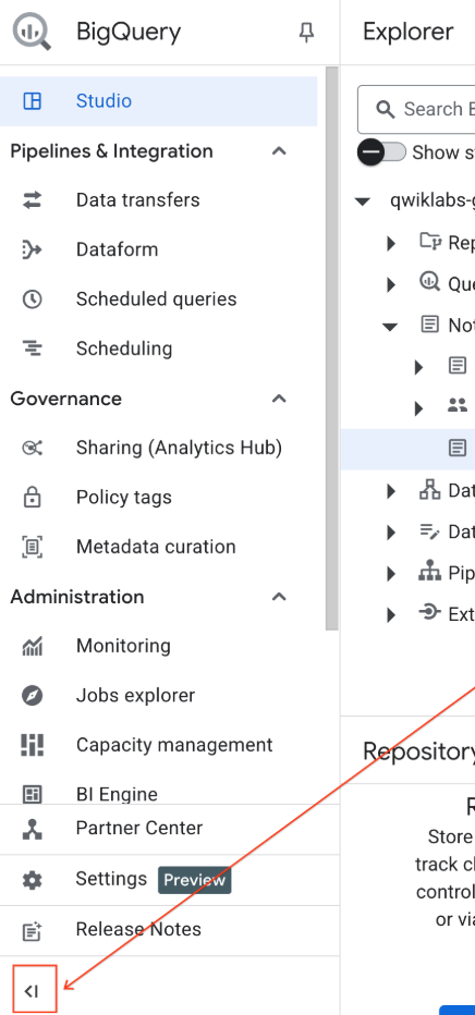
- Google Cloud Console में, नेविगेशन मेन्यू > BigQuery पर जाएं.
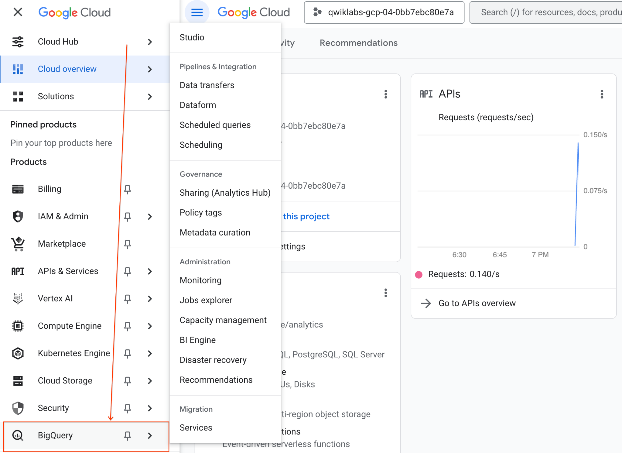
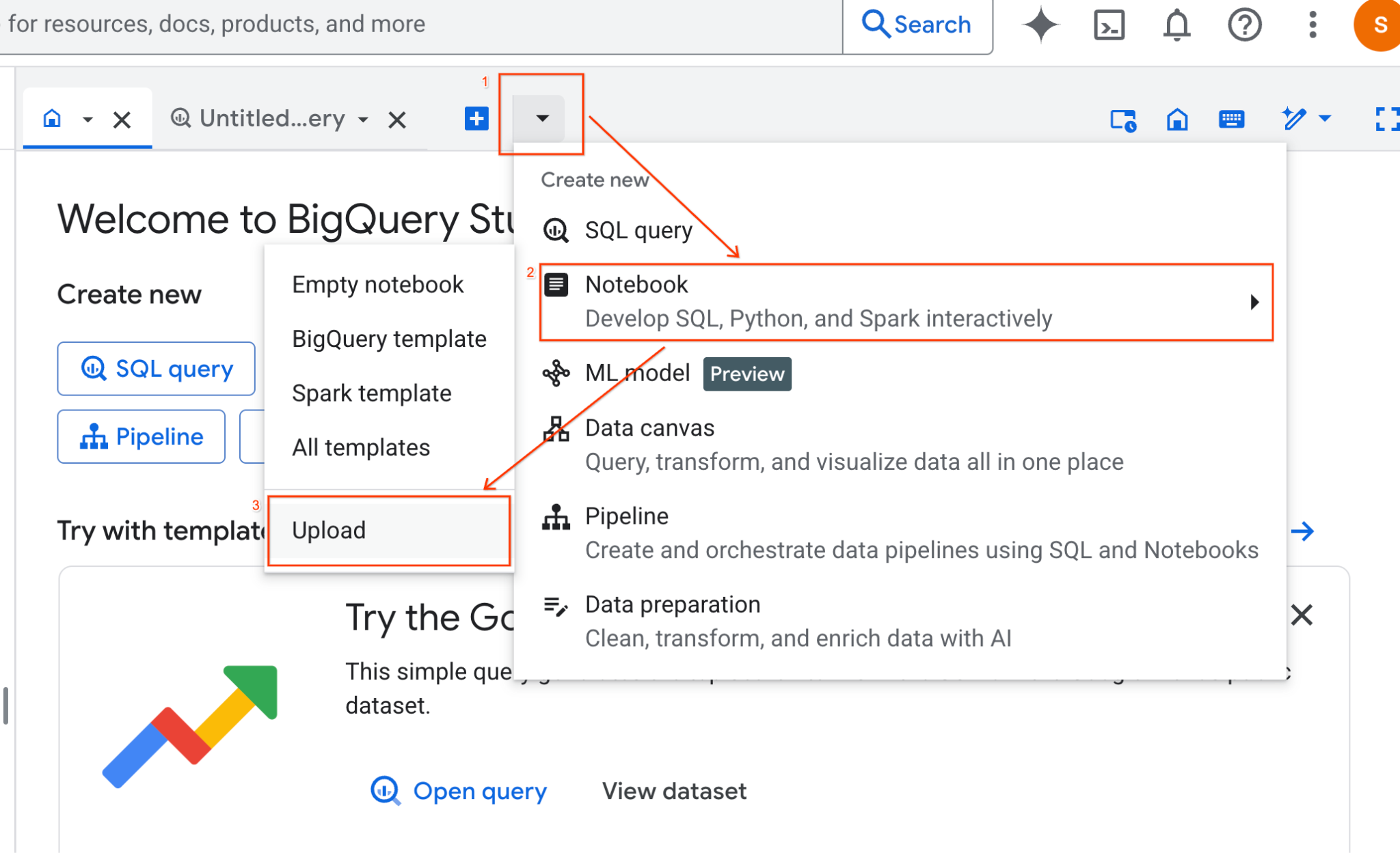
- BigQuery Studio के पैनल में, ड्रॉपडाउन ऐरो बटन पर क्लिक करें. इसके बाद, नोटबुक पर कर्सर घुमाएं और अपलोड करें को चुनें.
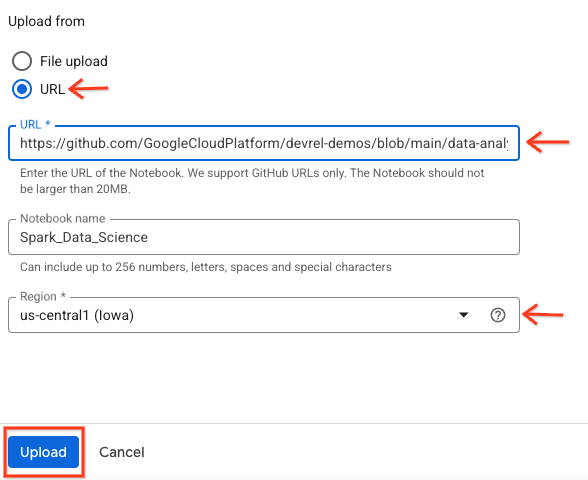
- यूआरएल रेडियो बटन चुनें और यह यूआरएल डालें:
https://github.com/GoogleCloudPlatform/devrel-demos/blob/main/data-analytics/dataproc-webinar/data-science/Spark_Data_Science.ipynb
- क्षेत्र को
us-central11पर सेट करें और अपलोड करें पर क्लिक करें.
- नोटबुक खोलने के लिए, अपने प्रोजेक्ट-आईडी के नाम वाले एक्सप्लोरर पैनल में मौजूद ड्रॉपडाउन ऐरो पर क्लिक करें. इसके बाद, नोटबुक के लिए, ड्रॉपडाउन पर क्लिक करें. नोटबुक
Spark_Data_Scienceपर क्लिक करें.
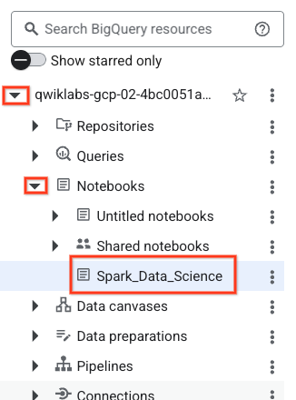
- ज़्यादा जगह पाने के लिए, BigQuery नेविगेशन मेन्यू और नोटबुक की विषय सूची को छोटा करें.
3. किसी रनटाइम से कनेक्ट करना और सेटअप का अतिरिक्त कोड चलाना
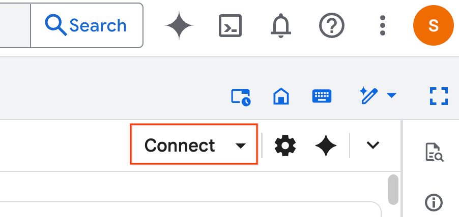
- कनेक्ट करें पर क्लिक करें. पॉप-अप में, अपने ईमेल खाते से Colab Enterprise को अनुमति दें. आपकी नोटबुक, रनटाइम से अपने-आप कनेक्ट हो जाएगी.
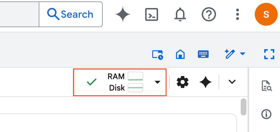
- रनटाइम तय होने के बाद, आपको यह दिखेगा:
- नोटबुक में, सेटअप सेक्शन तक स्क्रोल करें. यहां से शुरू करें.
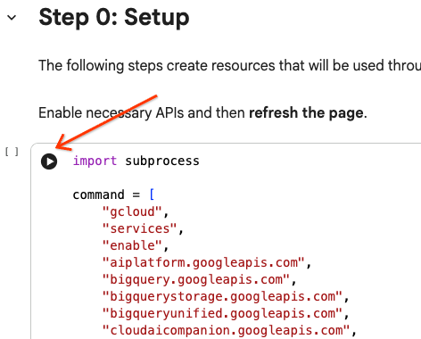
4. सेटअप कोड लागू करना
लैब को पूरा करने के लिए, अपने एनवायरमेंट को ज़रूरी Python लाइब्रेरी के साथ कॉन्फ़िगर करें. निजी Google ऐक्सेस को कॉन्फ़िगर करना. स्टोरेज बकेट बनाएं. BigQuery डेटासेट बनाएं. अपने प्रोजेक्ट आईडी को नोटबुक में कॉपी करें. कोई देश/इलाका चुनें. इस लैब के लिए, us-central1 क्षेत्र का इस्तेमाल करें.
कोड सेल को चलाने के लिए, सेल ब्लॉक में कर्सर घुमाएं और ऐरो पर क्लिक करें.
# Enable APIs
import subprocess

command = [
    "gcloud",
    "services",
    "enable",
    "aiplatform.googleapis.com",
    "bigquery.googleapis.com",
    "bigquerystorage.googleapis.com",
    "bigqueryunified.googleapis.com",
    "cloudaicompanion.googleapis.com",
    "dataproc.googleapis.com",
    "run.googleapis.com",
    "storage.googleapis.com"
]

result = subprocess.run(command, capture_output=True, text=True)
print(result.stdout)
print(result.stderr)

# Configure a PROJECT_ID and REGION
PROJECT_ID = "<YOUR_PROJECT_ID>"
REGION = "<YOUR_REGION>"

# Enable Private Google Access
import subprocess

command = [
    "gcloud",
    "compute",
    "networks",
    "subnets",
    "update",
    "default",
    f"--region={REGION}",
    "--enable-private-ip-google-access"
]

result = subprocess.run(command, capture_output=True, text=True)
print(result.stdout)
print(result.stderr)

# Create a Cloud Storage Bucket
from google.cloud import storage
from google.cloud.exceptions import NotFound

BUCKET_NAME = f"{PROJECT_ID}-demo"

storage_client = storage.Client(project=PROJECT_ID)
try:
    bucket = storage_client.get_bucket(BUCKET_NAME)
    print(f"Bucket {BUCKET_NAME} already exists.")
except NotFound:
    bucket = storage_client.create_bucket(BUCKET_NAME, location=REGION)
    print(f"Bucket {BUCKET_NAME} created.")


# Create a BigQuery dataset.
from google.cloud import bigquery

DATASET_ID = f"{PROJECT_ID}.demo"

client = bigquery.Client()

dataset = bigquery.Dataset(DATASET_ID)

dataset.location = REGION

dataset = client.create_dataset(dataset, exists_ok=True)
5. Google Cloud Serverless for Apache Spark से कनेक्शन बनाना
Spark Connect का इस्तेमाल करके, सर्वरलेस Spark सेशन से कनेक्ट किया जाता है. इससे इंटरैक्टिव Spark जॉब चलाए जा सकते हैं. बेहतर Spark परफ़ॉर्मेंस के लिए, Lightning Engine की मदद से रनटाइम को कॉन्फ़िगर किया जाता है. Lightning Engine, Apache Gluten और Velox का इस्तेमाल करके, वर्कलोड को तेज़ी से प्रोसेस करता है.
from google.cloud.dataproc_spark_connect import DataprocSparkSession
from google.cloud.dataproc_v1 import Session

session = Session()

session.runtime_config.version = "3.0"

# You can optionally configure Spark properties as well. See https://cloud.google.com/dataproc-serverless/docs/concepts/properties.
session.runtime_config.properties = {
  "dataproc.runtime": "premium",
  "spark.dataproc.engine": "lightningEngine",
}

# To avoid going over quota in this demo, cap the max number of Spark workers.
session.runtime_config.properties = {
    "spark.dynamicAllocation.maxExecutors": "4"
}

spark = (
    DataprocSparkSession.builder
      .appName("CustomSparkSession")
      .dataprocSessionConfig(session)
      .getOrCreate()
)
6. Gemini का इस्तेमाल करके, डेटा लोड करना और उसे एक्सप्लोर करना
इस सेक्शन में, आपको डेटा साइंस के किसी भी प्रोजेक्ट का पहला ज़रूरी चरण पूरा करना होता है: डेटा तैयार करना. इसके लिए, सबसे पहले BigQuery से Apache Spark dataframe में डेटा लोड करें.
# Load the tables
order_items = spark.read.format("bigquery").option("table", "bigquery-public-data.thelook_ecommerce.order_items").load()

users = spark.read.format("bigquery").option("table", "bigquery-public-data.thelook_ecommerce.users").load()

# Register temp tables
users.createOrReplaceTempView("users")
order_items.createOrReplaceTempView("order_items")

# Verify temp tables
spark.sql("SELECT * FROM order_items LIMIT 10").show()
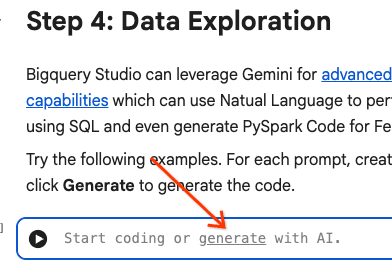
इसके बाद, Gemini का इस्तेमाल करके PySpark कोड जनरेट करें, ताकि डेटा को एक्सप्लोर किया जा सके और उसे बेहतर तरीके से समझा जा सके.
पहला प्रॉम्प्ट: PySpark का इस्तेमाल करके, उपयोगकर्ताओं की टेबल एक्सप्लोर करें और पहली 10 लाइनें दिखाएं.
# prompt:  Using PySpark, explore the users table and show the first 10 rows.

users.show(10)
दूसरा प्रॉम्प्ट: PySpark का इस्तेमाल करके, order_items टेबल एक्सप्लोर करें और पहली 10 लाइनें दिखाएं.
# prompt: Using PySpark, explore the order_items table and show the first 10 rows.

order_items.show(10)
तीसरा प्रॉम्प्ट: PySpark का इस्तेमाल करके, उपयोगकर्ताओं की टेबल में सबसे ज़्यादा बार दिखने वाले टॉप 5 देशों को दिखाएं. देश और हर देश के उपयोगकर्ताओं की संख्या दिखाएं.
# prompt: Using PySpark, show the top 5 most frequent countries in the users table. Display the country and the number of users from each country.

from pyspark.sql.functions import col, count

users.groupBy("country").agg(count("*").alias("user_count")).orderBy(col("user_count").desc()).limit(5).show()
चौथा प्रॉम्प्ट: PySpark का इस्तेमाल करके, order_items टेबल में मौजूद सामान की सेल में कीमत का औसत पता लगाएं.
# prompt: Using PySpark, find the average sale price of items in the order_items table.

from pyspark.sql import functions as F

average_sale_price = order_items.agg(F.avg("sale_price").alias("average_sale_price"))
average_sale_price.show()
पांचवां प्रॉम्प्ट: "users" टेबल का इस्तेमाल करके, देश बनाम ट्रैफ़िक सोर्स को प्लॉट करने के लिए कोड जनरेट करें. इसके लिए, प्लॉटिंग की सही लाइब्रेरी का इस्तेमाल करें.
# prompt: Using the table "users", generate code to plot country vs traffic source using a suitable plotting library.

sql = """
    SELECT
        country,
        traffic_source
    FROM
        `bigquery-public-data.thelook_ecommerce.users`
    WHERE country IS NOT NULL AND traffic_source IS NOT NULL
"""
project_id = "iceberg-summit-2025"
df = pandas_gbq.read_gbq(sql, project_id=project_id, dialect="standard")

import matplotlib.pyplot as plt
import seaborn as sns

# Group by country and traffic_source and count occurrences
df_grouped = df.groupby(['country', 'traffic_source']).size().reset_index(name='count')

# Create a pivot table for easier plotting
pivot_table = df_grouped.pivot(index='country', columns='traffic_source', values='count').fillna(0)

# Plotting
plt.figure(figsize=(15, 8))
pivot_table.plot(kind='bar', stacked=True, figsize=(15, 8))
plt.title('Traffic Source Distribution by Country')
plt.xlabel('Country')
plt.ylabel('Number of Users')
plt.xticks(rotation=90)
plt.legend(title='Traffic Source')
plt.tight_layout()
plt.show()
छठा प्रॉम्प्ट: "उम्र", "देश", "लिंग", "ट्रैफ़िक सोर्स" के डिस्ट्रिब्यूशन को दिखाने वाला हिस्टोग्राम बनाओ.
# prompt: Create a histogram showing the distribution of "age", "country", "gender", "traffic_source".

import matplotlib.pyplot as plt

# Convert Spark DataFrame to Pandas DataFrame for visualization
users_pd = users.toPandas()

# Create histograms for 'age', 'country', 'gender', 'traffic_source'
fig, axes = plt.subplots(2, 2, figsize=(15, 10))
fig.suptitle('Distribution of User Attributes')

# Age distribution
axes[0, 0].hist(users_pd['age'].dropna(), bins=20, edgecolor='black')
axes[0, 0].set_title('Age Distribution')
axes[0, 0].set_xlabel('Age')
axes[0, 0].set_ylabel('Number of Users')

# Country distribution
users_pd['country'].value_counts().head(10).plot(kind='bar', ax=axes[0, 1])
axes[0, 1].set_title('Top 10 Countries Distribution')
axes[0, 1].set_xlabel('Country')
axes[0, 1].set_ylabel('Number of Users')
axes[0, 1].tick_params(axis='x', rotation=45)

# Gender distribution
users_pd['gender'].value_counts().plot(kind='bar', ax=axes[1, 0])
axes[1, 0].set_title('Gender Distribution')
axes[1, 0].set_xlabel('Gender')
axes[1, 0].set_ylabel('Number of Users')
axes[1, 0].tick_params(axis='x', rotation=0)

# Traffic Source distribution
users_pd['traffic_source'].value_counts().head(10).plot(kind='bar', ax=axes[1, 1])
axes[1, 1].set_title('Top 10 Traffic Source Distribution')
axes[1, 1].set_xlabel('Traffic Source')
axes[1, 1].set_ylabel('Number of Users')
axes[1, 1].tick_params(axis='x', rotation=45)

plt.tight_layout(rect=[0, 0.03, 1, 0.95])
plt.show()
7. डेटा तैयार करना और फ़ीचर इंजीनियरिंग
इसके बाद, डेटा पर फ़ीचर इंजीनियरिंग की जाती है. सही कॉलम चुनें, डेटा को ज़्यादा सही डेटा टाइप में बदलें, और लेबल कॉलम की पहचान करें.
features = spark.sql("""
SELECT
  CAST(u.age AS DOUBLE) AS age,
  CAST(hash(u.country) AS BIGINT) * 1.0 AS country_hash,
  CAST(hash(u.gender) AS BIGINT) * 1.0 AS gender_hash,
  CAST(hash(u.traffic_source) AS BIGINT) * 1.0 AS traffic_source_hash,
  CASE WHEN COUNT(oi.id) > 0 THEN 1 ELSE 0 END AS label -- Changed label generation to count order items
FROM users AS u
LEFT JOIN order_items AS oi
ON u.id = oi.user_id
GROUP BY u.id, u.age, u.country, u.gender, u.traffic_source
""")
features.show()
8. लॉजिस्टिक रिग्रेशन मॉडल को ट्रेन करना
MLlib का इस्तेमाल करके, लॉजिस्टिक रिग्रेशन मॉडल को ट्रेन किया जाता है. सबसे पहले, डेटा को वेक्टर फ़ॉर्मैट में बदलने के लिए, VectorAssembler का इस्तेमाल किया जाता है. इसके बाद, StandardScaler बेहतर परफ़ॉर्मेंस के लिए, सुविधाओं वाले कॉलम को स्केल करता है. इसके बाद, LogisticRegression मॉडल का रेफ़रंस बनाया जाता है और हाइपरपैरामीटर तय किए जाते हैं. इन चरणों को Pipeline ऑब्जेक्ट में शामिल किया जाता है. इसके बाद, fit() फ़ंक्शन का इस्तेमाल करके मॉडल को ट्रेन किया जाता है. साथ ही, transform() फ़ंक्शन का इस्तेमाल करके डेटा में बदलाव किया जाता है.
from pyspark.ml.classification import LogisticRegression, LogisticRegressionModel
from pyspark.ml.evaluation import BinaryClassificationEvaluator
from pyspark.ml.feature import VectorAssembler, StandardScaler
from pyspark.ml.pipeline import Pipeline
from pyspark.ml.functions import array_to_vector

#Split Train and Test Data (80:20)
train_data, test_data = features.randomSplit([0.8, 0.2], seed=42)

# Initialize VectorAssembler
assembler = VectorAssembler(
    inputCols=["age", "country_hash", "gender_hash", "traffic_source_hash"],
    outputCol="assembled_features"
)

# Initialize StandardScaler
scaler = StandardScaler(inputCol="assembled_features", outputCol="scaled_features")

# Initialize Logistic Regression model
lr = LogisticRegression(
    maxIter=100,
    regParam=0.2,
    threshold=0.8,
    featuresCol="scaled_features",
    labelCol="label"
)

# Define pipeline
pipeline = Pipeline(stages=[assembler, scaler, lr])

# Fit the model
pipeline_model = pipeline.fit(train_data)

# Transform the dataset using the trained model
transformed_dataset = pipeline_model.transform(test_data)
transformed_dataset.show()
9. मॉडल का आकलन करना
बदले गए नए डेटासेट का आकलन करें. कर्व के नीचे का क्षेत्र (एयूसी) के लिए, आकलन मेट्रिक जनरेट करें.
# Model evaluation
eva = BinaryClassificationEvaluator(metricName="areaUnderPR")
aucPR = eva.evaluate(transformed_dataset)
print(f"AUC PR: {aucPR}")
इसके बाद, Gemini का इस्तेमाल करके, अपने मॉडल के आउटपुट को विज़ुअलाइज़ करने के लिए PySpark कोड जनरेट करें.
पहला प्रॉम्प्ट: प्रेसिज़न-रीकॉल (पीआर) कर्व को प्लॉट करने के लिए कोड जनरेट करो. मॉडल के अनुमानों से प्रेसिज़न और रीकॉल का हिसाब लगाएं. साथ ही, प्लॉटिंग के लिए सही लाइब्रेरी का इस्तेमाल करके पीआर कर्व दिखाएं.
# prompt: Generate code to plot the Precision-Recall (PR) curve. Calculate precision and recall from the model's predictions and display the PR curve using a suitable plotting library.

import matplotlib.pyplot as plt
from sklearn.metrics import precision_recall_curve, auc

# Extract predictions and labels
predictions = transformed_dataset.select("prediction", "label").toPandas()

# Calculate precision and recall
precision, recall, _ = precision_recall_curve(predictions["label"], predictions["prediction"])

# Calculate AUC-PR
pr_auc = auc(recall, precision)

# Plot the PR curve
plt.figure(figsize=(8, 6))
plt.plot(recall, precision, color='blue', lw=2, label=f'PR curve (AUC = {pr_auc:.2f})')
plt.xlabel('Recall')
plt.ylabel('Precision')
plt.title('Precision-Recall Curve')
plt.legend(loc='lower left')
plt.grid(True)
plt.show()
दूसरा प्रॉम्प्ट: कन्फ़्यूज़न मैट्रिक्स विज़ुअलाइज़ेशन बनाने के लिए कोड जनरेट करें. मॉडल के अनुमानों के आधार पर कन्फ़्यूज़न मैट्रिक्स का हिसाब लगाएं. साथ ही, इसे हीटमैप या ऐसी टेबल के तौर पर दिखाएं जिसमें सही पॉज़िटिव (टीपी), सही नेगेटिव (टीएन), गलत पॉज़िटिव (एफ़पी), और गलत नेगेटिव (एफ़एन) की संख्या दी गई हो.
# prompt: Generate code to create a confusion matrix visualization. Calculate the confusion matrix from the model's predictions and display it as a heat map or a table with counts of true positives (TP), true negatives (TN), false positives (FP), and false negatives (FN).

import pandas as pd
import seaborn as sns
import matplotlib.pyplot as plt
from sklearn.metrics import confusion_matrix

# Extract predictions and labels
predictions_and_labels = transformed_dataset.select("prediction", "label").toPandas()

# Calculate the confusion matrix
cm = confusion_matrix(predictions_and_labels["label"], predictions_and_labels["prediction"])

# Create a DataFrame for better visualization
cm_df = pd.DataFrame(cm,
                     index=['Actual Negative', 'Actual Positive'],
                     columns=['Predicted Negative', 'Predicted Positive'])

# Display the confusion matrix as a table
print("Confusion Matrix:")
print(cm_df)

# Display the confusion matrix as a heatmap
plt.figure(figsize=(8, 6))
sns.heatmap(cm_df, annot=True, fmt='d', cmap='Blues', cbar=False, linewidths=.5)
plt.title('Confusion Matrix')
plt.ylabel('Actual Label')
plt.xlabel('Predicted Label')
plt.show()

# Calculate and display TP, TN, FP, FN
TN, FP, FN, TP = cm.ravel()
print(f"
True Positives (TP): {TP}")
print(f"True Negatives (TN): {TN}")
print(f"False Positives (FP): {FP}")
print(f"False Negatives (FN): {FN}")
10. BigQuery में अनुमान लिखना
Gemini का इस्तेमाल करके, ऐसा कोड जनरेट करें जिससे आपकी अनुमानित वैल्यू को BigQuery डेटासेट में मौजूद नई टेबल में लिखा जा सके.
प्रॉम्प्ट: Spark का इस्तेमाल करके, बदले गए डेटासेट को BigQuery में लिखो.
# prompt: Using Spark, write the transformed dataset to BigQuery.

transformed_dataset.write.format("bigquery").option("table", f"{PROJECT_ID}.demo.predictions").mode("overwrite").save()
11. मॉडल को Cloud Storage में सेव करना
MLlib की नेटिव सुविधा का इस्तेमाल करके, अपने मॉडल को Cloud Storage में सेव करें. इन्फ़रेंस सर्वर, मॉडल को यहाँ से लोड करता है.
MODEL_PATH = "models/prediction_model"
pipeline_model.write().overwrite().save(f"gs://{BUCKET_NAME}/{MODEL_PATH}")
12. अनुमान लगाने वाला सर्वर बनाना
Cloud Run, बिना सर्वर के काम करने वाले वेब ऐप्लिकेशन को चलाने के लिए एक फ़्लेक्सिबल टूल है. यह उपयोगकर्ताओं को ज़्यादा से ज़्यादा सुविधाएँ देने के लिए, Docker कंटेनर का इस्तेमाल करता है. इस लैब के लिए, PySpark को चलाने वाले Flask ऐप्लिकेशन को चलाने के लिए Dockerfile कॉन्फ़िगर किया गया है. यह कंटेनर, Cloud Run पर चलता है. इससे इनपुट डेटा पर अनुमान लगाया जाता है. इसका कोड यहां देखा जा सकता है.
इन्फ़्रेंस सर्वर कोड के साथ रेपो क्लोन करें.
!git clone https://github.com/GoogleCloudPlatform/devrel-demos.git
Dockerfile देखें.
FROM python:3.12-slim

# Install OpenJDK-21 (Required for Spark)
RUN apt-get update && \
    apt-get install -y openjdk-21-jre-headless procps && \
    rm -rf /var/lib/apt/lists/*

ENV JAVA_HOME=/usr/lib/jvm/java-21-openjdk-amd64
ENV PORT=8080

WORKDIR /app

COPY requirements.txt .
RUN pip install --no-cache-dir -r requirements.txt

COPY main.py .

CMD ["gunicorn", "--bind", "0.0.0.0:8080", "--workers", "1", "--threads", "8", "--timeout", "0", "main:app"]
सर्वर के लिए Python कोड देखें.
import os
import json
import logging

from flask import Flask, request, jsonify
from google.cloud import storage
from pyspark.ml import PipelineModel
from pyspark.sql import SparkSession
from pyspark.sql.functions import hash, col

# Configure basic logging
logging.basicConfig(level=logging.INFO, format='%(asctime)s - %(levelname)s - %(message)s')

# --- Initialization: Spark and Model Loading ---
GCS_BUCKET = os.environ.get("GCS_BUCKET")
GCS_MODEL_PATH = os.environ.get("GCS_MODEL_PATH")
LOCAL_MODEL_PATH = "/tmp/model"

try:
    spark = SparkSession.builder \
        .appName("CloudRunSparkService") \
        .master("local[*]") \
        .getOrCreate()
    logging.info("Spark Session successfully initialized.")
except Exception as e:
    logging.error(f"Failed to initialize Spark Session: {e}")
    raise

def download_directory(bucket_name, prefix, local_path):
    """Downloads a directory from GCS to local filesystem."""
    storage_client = storage.Client()
    bucket = storage_client.get_bucket(bucket_name)
    blobs = list(bucket.list_blobs(prefix=prefix))

    if len(blobs) == 0:
        logging.error(f"No files found in GCS bucket {bucket_name} at prefix {prefix}")
        return

    for blob in blobs:
        if blob.name.endswith("/"): continue # Skip directories

        # Structure local paths
        relative_path = os.path.relpath(blob.name, prefix)
        local_file_path = os.path.join(local_path, relative_path)
        os.makedirs(os.path.dirname(local_file_path), exist_ok=True)

        blob.download_to_filename(local_file_path)
    print(f"Model downloaded to {local_path}")

# Load model
def load_model(LOCAL_MODEL_PATH, GCS_BUCKET, GCS_MODEL_PATH):
    """Download and load model on startup to avoid latency per request."""
    global MODEL
    if not os.path.exists(LOCAL_MODEL_PATH):
        download_directory(GCS_BUCKET, GCS_MODEL_PATH, LOCAL_MODEL_PATH)

    logging.info(f"Loading PySpark model from {GCS_MODEL_PATH}")
    # Load the Spark ML model
    try:
        MODEL = PipelineModel.load(LOCAL_MODEL_PATH)
        logging.info("Spark model loaded successfully.")
    except Exception as e:
        logging.error(f"Failed to load model: {e}")
        raise

# Load Model on Startup
load_model(LOCAL_MODEL_PATH, GCS_BUCKET, GCS_MODEL_PATH)

# --- Flask Application Setup ---
app = Flask(__name__)

@app.route('/predict', methods=['POST'])
def predict():
    """
    Handles incoming POST requests for inference.
    Expects JSON data that can be converted into a Spark DataFrame.
    """
    if MODEL is None:
        return jsonify({"error": "Model failed to load at startup."}), 500

    try:
        # 1. Get data from the request
        data = request.get_json()

        # 2. Check length of list
        data_len = len(data)
        cap = 100
        if data_len > cap:
            return jsonify({"error": f"Too many records. Count: {data_len}, Max: {cap}"}), 400

        # 2. Create Spark DataFrame
        df = spark.createDataFrame(data)

        # 3. Transform data
        input_df = df.select(
            col("age").cast("DOUBLE").alias("age"),
            (hash(col("country")).cast("BIGINT") * 1.0).alias("country_hash"),
            (hash(col("gender")).cast("BIGINT") * 1.0).alias("gender_hash"),
            (hash(col("traffic_source")).cast("BIGINT") * 1.0).alias("traffic_source_hash")
        )

        # 3. Perform Inference
        predictions_df = MODEL.transform(input_df)

        # 4. Prepare results (collect and serialize)
        results = [p.prediction for p in predictions_df.select("prediction").collect()]

        # 5. Return JSON response
        return jsonify({"predictions": results})

    except Exception as e:
        logging.error(f"An error occurred during prediction: {e}")
        #return jsonify({"error": str(e)}), 500
        raise e

# Gunicorn entry point uses 'app' from this file
if __name__ == '__main__':
    # Local testing only: Cloud Run uses Gunicorn/CMD command
    app.run(host='0.0.0.0', port=int(os.environ.get('PORT', 8080)))
इन्फ़रेंस सर्वर को डिप्लॉय करें.
import subprocess

command = [
    "gcloud",
    "run",
    "deploy",
    "inference-server",
    "--source",
    "/content/devrel-demos/data-analytics/dataproc-webinar/data-science/inference-server",
    "--region",
    f"{REGION}",
    "--port",
    "8080",
    "--memory",
    "2Gi",
    "--allow-unauthenticated",
    "--set-env-vars",
    f"GCS_BUCKET={BUCKET_NAME},GCS_MODEL_PATH={MODEL_PATH}",
    "--startup-probe",
    "tcpSocket.port=8080,initialDelaySeconds=240,failureThreshold=3,timeoutSeconds=240,periodSeconds=240"
]

result = subprocess.run(command, capture_output=True, text=True)
print(result.stdout)
print(result.stderr)
आउटपुट से अनुमान लगाने वाले सर्वर का यूआरएल कॉपी करके, नए वैरिएबल में चिपकाएं. यह https://inference-server-123456789.us-central1.run.app. की तरह ही होगा
INFERENCE_SERVER_URL = "<YOUR_SERVER_URL>"
इनफ़रेंस सर्वर की जांच करें.
import requests

age = "25.0"
country = "United States"
traffic_source = "Search"
gender = "F"

response = requests.post(
    f"{INFERENCE_SERVER_URL}/predict",
    json=[{"age": age, "country": country, "traffic_source": traffic_source, "gender": gender}],
    headers={"Content-Type": "application/json"}
)

print(response.json())
आउटपुट 1.0 या 0.0 होना चाहिए.
{'predictions': [1.0]}
13. किसी एजेंट को कॉन्फ़िगर करना
अनुमान लगाने वाले एजेंट को बनाने के लिए, एजेंट इंजन का इस्तेमाल करें. Agent Engine, Vertex AI Platform का हिस्सा है. यह सेवाओं का एक ऐसा सेट है जो डेवलपर को प्रोडक्शन में एआई एजेंट डिप्लॉय करने, मैनेज करने, और बड़े पैमाने पर उपलब्ध कराने की सुविधा देता है. इसमें कई टूल हैं. जैसे, एजेंटों का आकलन करना, सेशन के कॉन्टेक्स्ट, और कोड को लागू करना. यह कई लोकप्रिय एजेंटिक फ़्रेमवर्क के साथ काम करता है. इनमें एजेंट डेवलपमेंट किट (एडीके) भी शामिल है. ADK एक ओपन सोर्स एजेंटिक फ़्रेमवर्क है. इसे Gemini और Google के नेटवर्क के साथ इस्तेमाल करने के लिए बनाया और ऑप्टिमाइज़ किया गया है. हालांकि, यह मॉडल-अग्नोस्टिक है. इसे इस तरह से डिज़ाइन किया गया है कि एजेंट डेवलपमेंट, सॉफ़्टवेयर डेवलपमेंट की तरह लगे.
Vertex AI क्लाइंट को शुरू करें.
import vertexai
from vertexai import agent_engines # For the prebuilt templates

client = vertexai.Client(  # For service interactions via client.agent_engines
    project=f"{PROJECT_ID}",
    location=f"{REGION}",
)
डिप्लॉय किए गए मॉडल से क्वेरी करने के लिए, एक फ़ंक्शन तय करें.
def predict_purchase(
    age: str = "25.0",
    country: str = "United States",
    traffic_source: str = "Search",
    gender: str = "M",
):
    """Predicts whether or not a user will purchase a product.

    Args:
        age: The age of the user.
        country: The country of the user. One of: "China", "Poland", "Germany", "United States", "Spain", "United Kingdom", "España", "Japan", "Brasil", "Colombia", "Belgium", "South Korea", "Austria", "France", "Australia".
        Traffic_source: The source of the user's traffic. One of: "Display", "Email", "Search", "Organic", "Facebook".
        gender: The gender of the user. One of: "M" or "F".

    Returns:
        True if the model output is 1.0, False otherwise.
    """
    import requests
    response = requests.post(
        f"{INFERENCE_SERVER_URL}/predict",
        json=[{"age": age, "country": country, "traffic_source": traffic_source, "gender": gender}],
        headers={"Content-Type": "application/json"}
    )
    return response.json()
सैंपल पैरामीटर पास करके फ़ंक्शन की जांच करें.
predict_purchase(age=25.0, country="United States", traffic_source="Search", gender="M")
ADK का इस्तेमाल करके, नीचे दिए गए एजेंट को तय करें और predict_purchase फ़ंक्शन को टूल के तौर पर उपलब्ध कराएं.
from google.adk.agents import Agent
from vertexai import agent_engines

agent = Agent(
   model="gemini-2.5-flash",
   name='purchase_prediction_agent',
   tools=[predict_purchase]
)
कोई क्वेरी डालकर, एजेंट को स्थानीय तौर पर टेस्ट करें.
app = agent_engines.AdkApp(agent=agent)
async for event in app.async_stream_query(
    user_id="123",
    message="Will a 25 yo male from the United States who came from Search make a purchase? Strictly output 'yes' or 'no'.",
):
    try:
        print(event['content']['parts'][0]['text'])
    except:
      continue
मॉडल को एजेंट इंजन में डिप्लॉय करें.
remote_agent = client.agent_engines.create(
    agent=app,
    config={
        "requirements": ["google-cloud-aiplatform[agent_engines,adk]"],
        "staging_bucket": f"gs://{BUCKET_NAME}",
        "display_name": "purchase-predictor",
        "description": "Agent that predicts whether or not a user will purchase a product.",
    }
)
इसके बाद, डिप्लॉय किए गए मॉडल को Cloud Console में देखें.
मॉडल से फिर से क्वेरी करें. अब यह लोकल वर्शन के बजाय, डिप्लॉय किए गए एजेंट की ओर इशारा करता है.
async for event in remote_agent.async_stream_query(
    user_id="123",
    message="Will a 25 yo male from the United States who came from Search make a purchase? Strictly output 'yes' or 'no'.",
):
    try:
        print(event['content']['parts'][0]['text'])
    except:
      continue
14. व्यवस्थित करें
आपने Google Cloud के जो भी संसाधन बनाए हैं उन्हें मिटाएं. इस तरह की क्लीनअप कमांड चलाना, आने वाले समय में शुल्क लगने से बचने के लिए सबसे सही तरीका है.
# Delete the deployed agent.
remote_agent.delete(force=True)

# Delete the inference server.
import subprocess

command = [
    "gcloud",
    "run",
    "services",
    "delete",
    "inference-server",
    "--region",
    f"{REGION}",
    "--quiet"
]

subprocess.run(command, capture_output=True, text=True)

# Delete the BigQuery dataset.
bigquery_client = bigquery.Client()

bigquery_client.delete_dataset(
    f"{PROJECT_ID}.demo", delete_contents=True, not_found_ok=True
)

# Delete the Storage bucket.
storage_client = storage.Client()

bucket = storage_client.get_bucket(BUCKET_NAME)
bucket.delete_blobs(list(bucket.list_blobs()))
bucket.delete()
15. बधाई हो!
आपने कर दिखाया! इस कोडलैब में, आपने ये काम किए:
- डेटा साइंस वर्कफ़्लो को चलाने के लिए, BigQuery Studio नोटबुक का इस्तेमाल किया.
- Google Cloud Serverless for Apache Spark का इस्तेमाल करके, Apache Spark से कनेक्शन बनाया गया है. साथ ही, इसे Spark Connect की मदद से चलाया जाता है.
- Lightning Engine का इस्तेमाल करके, Apache Spark के वर्कलोड को 4.3 गुना तक बढ़ाया गया.
- Apache Spark और BigQuery के बीच पहले से मौजूद इंटिग्रेशन का इस्तेमाल करके, BigQuery से डेटा लोड किया गया.
- Gemini की मदद से कोड जनरेट करने की सुविधा का इस्तेमाल करके, डेटा एक्सप्लोर किया गया.
- Apache Spark के डेटा प्रोसेसिंग फ़्रेमवर्क का इस्तेमाल करके, फ़ीचर इंजीनियरिंग की गई.
- Apache Spark की नेटिव मशीन लर्निंग लाइब्रेरी, MLlib का इस्तेमाल करके, क्लासिफ़िकेशन मॉडल को ट्रेन किया और उसका आकलन किया.
- Flask और Cloud Run का इस्तेमाल करके, क्लासिफ़िकेशन मॉडल के लिए अनुमान सर्वर डिप्लॉय किया गया
- Agent Engine और Agent Development Kit (ADK) का इस्तेमाल करके, आम भाषा में क्वेरी करने के लिए एजेंट को डिप्लॉय किया गया हो,
आगे क्या करना है?
- Google Cloud Serverless for Apache Spark के बारे में ज़्यादा जानें.
- Cloud Run को कॉन्फ़िगर करने का तरीका जानें.
- एजेंट इंजन के बारे में पढ़ें.