Spark を使用したデータ サイエンス

1. 概要

架空の衣料品 e コマース小売業者である TheLook は、顧客、商品、注文、ロジスティクス、ウェブ イベント、デジタル マーケティング キャンペーンに関するデータを BigQuery に保存しています。同社は、チームの既存の SQL と PySpark の専門知識を活用して、Apache Spark を使用してこのデータを分析したいと考えています。

TheLook は、Spark のインフラストラクチャのプロビジョニングやチューニングを手動で行う必要がない、クラスタ管理ではなくワークロードに集中できる自動スケーリング ソリューションを求めています。また、BigQuery Studio 環境内で Spark と BigQuery を統合するのに必要な労力を最小限に抑えたいと考えています。

このラボでは、PySpark を使用してロジスティック回帰分類子を構築し、BigQuery Studio のネイティブ ノートブック統合と AI 機能を利用してデータを探索することで、ユーザーが購入するかどうかを予測します。このモデルを推論サーバーにデプロイし、自然言語を使用してモデルにクエリを実行するエージェントを作成します。

前提条件

このラボを開始する前に、以下について理解しておく必要があります。

• 基本的な SQL と Python のプログラミング。
• Jupyter ノートブックで Python コードを実行する。
• 分散コンピューティングに関する基本的な知識

目標

• BigQuery Studio ノートブックを使用して、データ サイエンス ワークフローを実行する。
• Apache Spark 向け Google Cloud Serverless を使用し、Spark Connect を利用して Apache Spark への接続を作成します。
• Lightning Engine を使用して、Apache Spark ワークロードを最大 4.3 倍高速化します。
• Apache Spark と BigQuery の組み込み統合を使用して、BigQuery からデータを読み込みます。
• Gemini アシストによるコード生成を使用してデータを探索する。
• Apache Spark のデータ処理フレームワークを使用して特徴量エンジニアリングを実行します。
• Apache Spark のネイティブ ML ライブラリである MLlib を使用して、分類モデルをトレーニングして評価します。
• Flask と Cloud Run を使用して分類モデルの推論サーバーをデプロイする
• Agent Engine と Agent Development Kit（ADK）を使用して、自然言語で推論サーバーにクエリを実行するエージェントをデプロイする。

2. Colab ランタイム環境に接続する

Google Cloud プロジェクトを特定する

Google Cloud プロジェクトを作成します。既存のものを利用してもかまいません。

推奨 API を有効にする:

こちらをクリックして、次の API を有効にします。

• aiplatform.googleapis.com
• bigquery.googleapis.com
• bigquerystorage.googleapis.com
• bigqueryunified.googleapis.com
• cloudaicompanion.googleapis.com
• dataproc.googleapis.com
• storage.googleapis.com
• run.googleapis.com

UI の操作:

1. Google Cloud コンソールで、ナビゲーション メニュー > [BigQuery] に移動します。

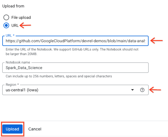
2. BigQuery Studio ペインで、プルダウン矢印ボタンをクリックし、[ノートブック] にカーソルを合わせて、[アップロード] を選択します。

3. [URL] ラジオボタンを選択し、次の URL を入力します。

https://github.com/GoogleCloudPlatform/devrel-demos/blob/main/data-analytics/dataproc-webinar/data-science/Spark_Data_Science.ipynb

4. リージョンを us-central11 に設定し、[アップロード] をクリックします。

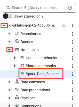
5. ノートブックを開くには、[エクスプローラ] ペインでプロジェクト ID の名前の横にあるプルダウン矢印をクリックします。[ノートブック] のプルダウンをクリックします。ノートブック Spark_Data_Science をクリックします。

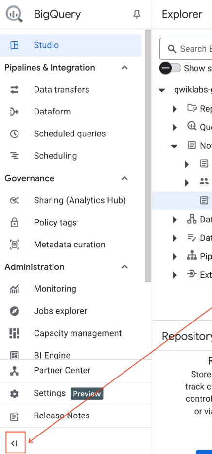
6. BigQuery ナビゲーション メニューとノートブックの目次を折りたたんで、スペースを広げます。

3. ランタイムに接続して追加のセットアップ コードを実行する

1. [接続] をクリックします。ポップアップで、メール アカウントを使用して Colab Enterprise を承認します。ノートブックはランタイムに自動的に接続されます。

注: この処理が完了するまでに数分かかることがあります。

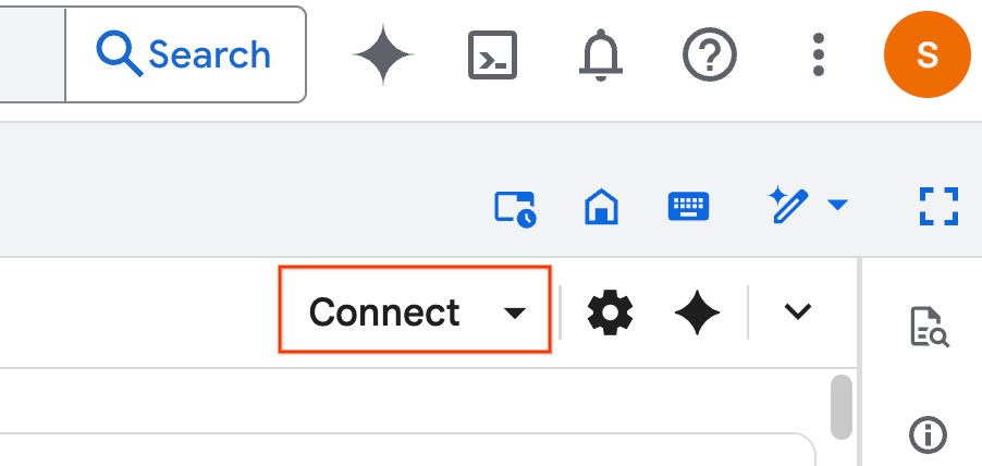
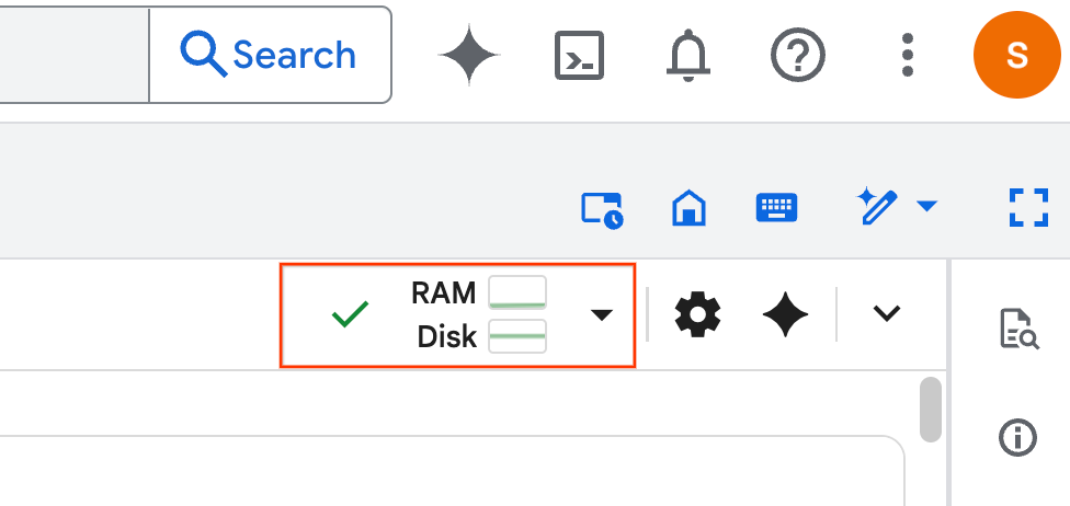
2. ランタイムが確立されると、次のように表示されます。

3. ノートブック内で、[設定] セクションまでスクロールします。こちらから始めましょう。

注: ノートブックを開いて準備ができたら、主に Colab 環境内で作業します。このノートブックには、すべてのコードと、ワークフロー全体のセルごとの詳細な説明が含まれています。このラボは概要ガイドとして、進捗状況を把握するのに役立つ簡単な概要を提供します。ここで Codelab を終了してもかまいません。

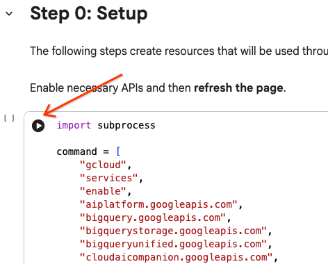
4. セットアップ コードを実行する

ラボを完了するために必要な Python ライブラリを使用して環境を構成します。プライベート Google アクセスを構成します。Storage バケットを作成します。BigQuery データセットを作成します。プロジェクト ID をノートブックにコピーします。リージョンを選択します。このラボでは、us-central1 リージョンを使用します。

コードセルを実行するには、セルブロック内にカーソルを合わせて矢印をクリックします。

# Enable APIs
import subprocess

command = [
    "gcloud",
    "services",
    "enable",
    "aiplatform.googleapis.com",
    "bigquery.googleapis.com",
    "bigquerystorage.googleapis.com",
    "bigqueryunified.googleapis.com",
    "cloudaicompanion.googleapis.com",
    "dataproc.googleapis.com",
    "run.googleapis.com",
    "storage.googleapis.com"
]

result = subprocess.run(command, capture_output=True, text=True)
print(result.stdout)
print(result.stderr)

# Configure a PROJECT_ID and REGION
PROJECT_ID = "<YOUR_PROJECT_ID>"
REGION = "<YOUR_REGION>"

# Enable Private Google Access
import subprocess

command = [
    "gcloud",
    "compute",
    "networks",
    "subnets",
    "update",
    "default",
    f"--region={REGION}",
    "--enable-private-ip-google-access"
]

result = subprocess.run(command, capture_output=True, text=True)
print(result.stdout)
print(result.stderr)

# Create a Cloud Storage Bucket
from google.cloud import storage
from google.cloud.exceptions import NotFound

BUCKET_NAME = f"{PROJECT_ID}-demo"

storage_client = storage.Client(project=PROJECT_ID)
try:
    bucket = storage_client.get_bucket(BUCKET_NAME)
    print(f"Bucket {BUCKET_NAME} already exists.")
except NotFound:
    bucket = storage_client.create_bucket(BUCKET_NAME, location=REGION)
    print(f"Bucket {BUCKET_NAME} created.")


# Create a BigQuery dataset.
from google.cloud import bigquery

DATASET_ID = f"{PROJECT_ID}.demo"

client = bigquery.Client()

dataset = bigquery.Dataset(DATASET_ID)

dataset.location = REGION

dataset = client.create_dataset(dataset, exists_ok=True)

5. Apache Spark 向け Google Cloud Serverless への接続を作成する

Spark Connect を使用して、サーバーレス Spark セッションに接続し、インタラクティブ Spark ジョブを実行します。高度な Spark パフォーマンスを実現するために、Lightning Engine を使用してランタイムを構成します。Lightning Engine は、Apache Gluten と Velox を使用してワークロードを高速化することで機能します。

from google.cloud.dataproc_spark_connect import DataprocSparkSession
from google.cloud.dataproc_v1 import Session

session = Session()

session.runtime_config.version = "3.0"

# You can optionally configure Spark properties as well. See https://cloud.google.com/dataproc-serverless/docs/concepts/properties.
session.runtime_config.properties = {
  "dataproc.runtime": "premium",
  "spark.dataproc.engine": "lightningEngine",
}

# To avoid going over quota in this demo, cap the max number of Spark workers.
session.runtime_config.properties = {
    "spark.dynamicAllocation.maxExecutors": "4"
}

spark = (
    DataprocSparkSession.builder
      .appName("CustomSparkSession")
      .dataprocSessionConfig(session)
      .getOrCreate()
)

6. Gemini を使用してデータを読み込み、探索する

このセクションでは、データ サイエンス プロジェクトの最初の重要なステップであるデータの準備について説明します。まず、BigQuery から Apache Spark DataFrame にデータを読み込みます。

# Load the tables
order_items = spark.read.format("bigquery").option("table", "bigquery-public-data.thelook_ecommerce.order_items").load()

users = spark.read.format("bigquery").option("table", "bigquery-public-data.thelook_ecommerce.users").load()

# Register temp tables
users.createOrReplaceTempView("users")
order_items.createOrReplaceTempView("order_items")

# Verify temp tables
spark.sql("SELECT * FROM order_items LIMIT 10").show()

次に、Gemini を使用して PySpark コードを生成し、データを探索して理解を深めます。

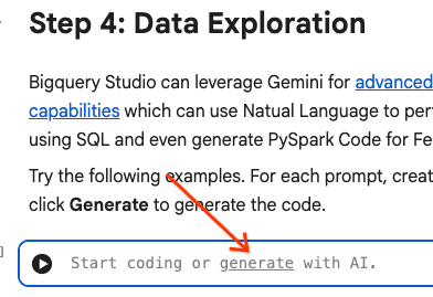
プロンプト 1: PySpark を使用して、users テーブルを調べ、最初の 10 行を表示します。

# prompt:  Using PySpark, explore the users table and show the first 10 rows.

users.show(10)

プロンプト 2: PySpark を使用して order_items テーブルを調べ、最初の 10 行を表示します。

# prompt: Using PySpark, explore the order_items table and show the first 10 rows.

order_items.show(10)

プロンプト 3: PySpark を使用して、users テーブルで最も頻繁に表示される上位 5 か国を表示します。国と、各国のユーザー数を表示します。

# prompt: Using PySpark, show the top 5 most frequent countries in the users table. Display the country and the number of users from each country.

from pyspark.sql.functions import col, count

users.groupBy("country").agg(count("*").alias("user_count")).orderBy(col("user_count").desc()).limit(5).show()

プロンプト 4: PySpark を使用して、order_items テーブル内のアイテムの平均セール価格を求めます。

# prompt: Using PySpark, find the average sale price of items in the order_items table.

from pyspark.sql import functions as F

average_sale_price = order_items.agg(F.avg("sale_price").alias("average_sale_price"))
average_sale_price.show()

プロンプト 5: 「users」テーブルを使用して、適切なプロット ライブラリを使用して国とトラフィック ソースをプロットするコードを生成します。

# prompt: Using the table "users", generate code to plot country vs traffic source using a suitable plotting library.

sql = """
    SELECT
        country,
        traffic_source
    FROM
        `bigquery-public-data.thelook_ecommerce.users`
    WHERE country IS NOT NULL AND traffic_source IS NOT NULL
"""
project_id = "iceberg-summit-2025"
df = pandas_gbq.read_gbq(sql, project_id=project_id, dialect="standard")

import matplotlib.pyplot as plt
import seaborn as sns

# Group by country and traffic_source and count occurrences
df_grouped = df.groupby(['country', 'traffic_source']).size().reset_index(name='count')

# Create a pivot table for easier plotting
pivot_table = df_grouped.pivot(index='country', columns='traffic_source', values='count').fillna(0)

# Plotting
plt.figure(figsize=(15, 8))
pivot_table.plot(kind='bar', stacked=True, figsize=(15, 8))
plt.title('Traffic Source Distribution by Country')
plt.xlabel('Country')
plt.ylabel('Number of Users')
plt.xticks(rotation=90)
plt.legend(title='Traffic Source')
plt.tight_layout()
plt.show()

プロンプト 6: 「年齢」、「国」、「性別」、「トラフィック ソース」の分布を示すヒストグラムを作成します。

# prompt: Create a histogram showing the distribution of "age", "country", "gender", "traffic_source".

import matplotlib.pyplot as plt

# Convert Spark DataFrame to Pandas DataFrame for visualization
users_pd = users.toPandas()

# Create histograms for 'age', 'country', 'gender', 'traffic_source'
fig, axes = plt.subplots(2, 2, figsize=(15, 10))
fig.suptitle('Distribution of User Attributes')

# Age distribution
axes[0, 0].hist(users_pd['age'].dropna(), bins=20, edgecolor='black')
axes[0, 0].set_title('Age Distribution')
axes[0, 0].set_xlabel('Age')
axes[0, 0].set_ylabel('Number of Users')

# Country distribution
users_pd['country'].value_counts().head(10).plot(kind='bar', ax=axes[0, 1])
axes[0, 1].set_title('Top 10 Countries Distribution')
axes[0, 1].set_xlabel('Country')
axes[0, 1].set_ylabel('Number of Users')
axes[0, 1].tick_params(axis='x', rotation=45)

# Gender distribution
users_pd['gender'].value_counts().plot(kind='bar', ax=axes[1, 0])
axes[1, 0].set_title('Gender Distribution')
axes[1, 0].set_xlabel('Gender')
axes[1, 0].set_ylabel('Number of Users')
axes[1, 0].tick_params(axis='x', rotation=0)

# Traffic Source distribution
users_pd['traffic_source'].value_counts().head(10).plot(kind='bar', ax=axes[1, 1])
axes[1, 1].set_title('Top 10 Traffic Source Distribution')
axes[1, 1].set_xlabel('Traffic Source')
axes[1, 1].set_ylabel('Number of Users')
axes[1, 1].tick_params(axis='x', rotation=45)

plt.tight_layout(rect=[0, 0.03, 1, 0.95])
plt.show()

7. データの準備と特徴量エンジニアリング

次に、データに対して特徴量エンジニアリングを実行します。適切な列を選択し、データをより適切なデータ型に変換して、ラベル列を特定します。

features = spark.sql("""
SELECT
  CAST(u.age AS DOUBLE) AS age,
  CAST(hash(u.country) AS BIGINT) * 1.0 AS country_hash,
  CAST(hash(u.gender) AS BIGINT) * 1.0 AS gender_hash,
  CAST(hash(u.traffic_source) AS BIGINT) * 1.0 AS traffic_source_hash,
  CASE WHEN COUNT(oi.id) > 0 THEN 1 ELSE 0 END AS label -- Changed label generation to count order items
FROM users AS u
LEFT JOIN order_items AS oi
ON u.id = oi.user_id
GROUP BY u.id, u.age, u.country, u.gender, u.traffic_source
""")
features.show()

8. ロジスティック回帰モデルをトレーニングする

MLlib を使用して、ロジスティック回帰モデルをトレーニングします。まず、VectorAssembler を使用してデータをベクトル形式に変換します。次に、StandardScaler はパフォーマンスを向上させるために特徴列をスケーリングします。次に、LogisticRegression モデルへの参照を作成し、ハイパーパラメータを定義します。これらの手順を Pipeline オブジェクトに結合し、fit() 関数を使用してモデルをトレーニングし、transform() 関数を使用してデータを変換します。

from pyspark.ml.classification import LogisticRegression, LogisticRegressionModel
from pyspark.ml.evaluation import BinaryClassificationEvaluator
from pyspark.ml.feature import VectorAssembler, StandardScaler
from pyspark.ml.pipeline import Pipeline
from pyspark.ml.functions import array_to_vector

#Split Train and Test Data (80:20)
train_data, test_data = features.randomSplit([0.8, 0.2], seed=42)

# Initialize VectorAssembler
assembler = VectorAssembler(
    inputCols=["age", "country_hash", "gender_hash", "traffic_source_hash"],
    outputCol="assembled_features"
)

# Initialize StandardScaler
scaler = StandardScaler(inputCol="assembled_features", outputCol="scaled_features")

# Initialize Logistic Regression model
lr = LogisticRegression(
    maxIter=100,
    regParam=0.2,
    threshold=0.8,
    featuresCol="scaled_features",
    labelCol="label"
)

# Define pipeline
pipeline = Pipeline(stages=[assembler, scaler, lr])

# Fit the model
pipeline_model = pipeline.fit(train_data)

# Transform the dataset using the trained model
transformed_dataset = pipeline_model.transform(test_data)
transformed_dataset.show()

9. モデルの評価

新しく変換したデータセットを評価します。評価指標の曲線下面積（AUC）を生成します。

# Model evaluation
eva = BinaryClassificationEvaluator(metricName="areaUnderPR")
aucPR = eva.evaluate(transformed_dataset)
print(f"AUC PR: {aucPR}")

次に、Gemini を使用して PySpark コードを生成し、モデル出力を可視化します。

プロンプト 1: 適合率 / 再現率（PR）曲線をプロットするコードを生成します。モデルの予測から適合率と再現率を計算し、適切なプロット ライブラリを使用して PR 曲線を表示します。

# prompt: Generate code to plot the Precision-Recall (PR) curve. Calculate precision and recall from the model's predictions and display the PR curve using a suitable plotting library.

import matplotlib.pyplot as plt
from sklearn.metrics import precision_recall_curve, auc

# Extract predictions and labels
predictions = transformed_dataset.select("prediction", "label").toPandas()

# Calculate precision and recall
precision, recall, _ = precision_recall_curve(predictions["label"], predictions["prediction"])

# Calculate AUC-PR
pr_auc = auc(recall, precision)

# Plot the PR curve
plt.figure(figsize=(8, 6))
plt.plot(recall, precision, color='blue', lw=2, label=f'PR curve (AUC = {pr_auc:.2f})')
plt.xlabel('Recall')
plt.ylabel('Precision')
plt.title('Precision-Recall Curve')
plt.legend(loc='lower left')
plt.grid(True)
plt.show()

プロンプト 2: 混同行列の可視化を作成するコードを生成します。モデルの予測から混同行列を計算し、真陽性（TP）、真陰性（TN）、偽陽性（FP）、偽陰性（FN）の数を含むヒートマップまたは表として表示します。

# prompt: Generate code to create a confusion matrix visualization. Calculate the confusion matrix from the model's predictions and display it as a heat map or a table with counts of true positives (TP), true negatives (TN), false positives (FP), and false negatives (FN).

import pandas as pd
import seaborn as sns
import matplotlib.pyplot as plt
from sklearn.metrics import confusion_matrix

# Extract predictions and labels
predictions_and_labels = transformed_dataset.select("prediction", "label").toPandas()

# Calculate the confusion matrix
cm = confusion_matrix(predictions_and_labels["label"], predictions_and_labels["prediction"])

# Create a DataFrame for better visualization
cm_df = pd.DataFrame(cm,
                     index=['Actual Negative', 'Actual Positive'],
                     columns=['Predicted Negative', 'Predicted Positive'])

# Display the confusion matrix as a table
print("Confusion Matrix:")
print(cm_df)

# Display the confusion matrix as a heatmap
plt.figure(figsize=(8, 6))
sns.heatmap(cm_df, annot=True, fmt='d', cmap='Blues', cbar=False, linewidths=.5)
plt.title('Confusion Matrix')
plt.ylabel('Actual Label')
plt.xlabel('Predicted Label')
plt.show()

# Calculate and display TP, TN, FP, FN
TN, FP, FN, TP = cm.ravel()
print(f"
True Positives (TP): {TP}")
print(f"True Negatives (TN): {TN}")
print(f"False Positives (FP): {FP}")
print(f"False Negatives (FN): {FN}")

10. 予測を BigQuery に書き込む

Gemini を使用して、BigQuery データセットの新しいテーブルに予測を書き込むコードを生成します。

プロンプト: Spark を使用して、変換されたデータセットを BigQuery に書き込みます。

# prompt: Using Spark, write the transformed dataset to BigQuery.

transformed_dataset.write.format("bigquery").option("table", f"{PROJECT_ID}.demo.predictions").mode("overwrite").save()

11. モデルを Cloud Storage に保存する

MLlib のネイティブ機能を使用して、モデルを Cloud Storage に保存します。推論サーバーはここからモデルを読み込みます。

MODEL_PATH = "models/prediction_model"
pipeline_model.write().overwrite().save(f"gs://{BUCKET_NAME}/{MODEL_PATH}")

12. 推論サーバーを作成する

Cloud Run は、サーバーレス ウェブアプリを実行するための柔軟なツールです。Docker コンテナを使用して、ユーザーに最大限のカスタマイズ性を提供します。このラボでは、PySpark を利用する Flask アプリを実行するように Dockerfile が構成されています。このコンテナは Cloud Run で実行され、入力データに対して推論を行います。コードについては、こちらをご覧ください。

推論サーバーのコードが含まれるリポジトリのクローンを作成します。

!git clone https://github.com/GoogleCloudPlatform/devrel-demos.git

Dockerfile を表示します。

FROM python:3.12-slim

# Install OpenJDK-21 (Required for Spark)
RUN apt-get update && \
    apt-get install -y openjdk-21-jre-headless procps && \
    rm -rf /var/lib/apt/lists/*

ENV JAVA_HOME=/usr/lib/jvm/java-21-openjdk-amd64
ENV PORT=8080

WORKDIR /app

COPY requirements.txt .
RUN pip install --no-cache-dir -r requirements.txt

COPY main.py .

CMD ["gunicorn", "--bind", "0.0.0.0:8080", "--workers", "1", "--threads", "8", "--timeout", "0", "main:app"]

サーバーの Python コードを表示します。

import os
import json
import logging

from flask import Flask, request, jsonify
from google.cloud import storage
from pyspark.ml import PipelineModel
from pyspark.sql import SparkSession
from pyspark.sql.functions import hash, col

# Configure basic logging
logging.basicConfig(level=logging.INFO, format='%(asctime)s - %(levelname)s - %(message)s')

# --- Initialization: Spark and Model Loading ---
GCS_BUCKET = os.environ.get("GCS_BUCKET")
GCS_MODEL_PATH = os.environ.get("GCS_MODEL_PATH")
LOCAL_MODEL_PATH = "/tmp/model"

try:
    spark = SparkSession.builder \
        .appName("CloudRunSparkService") \
        .master("local[*]") \
        .getOrCreate()
    logging.info("Spark Session successfully initialized.")
except Exception as e:
    logging.error(f"Failed to initialize Spark Session: {e}")
    raise

def download_directory(bucket_name, prefix, local_path):
    """Downloads a directory from GCS to local filesystem."""
    storage_client = storage.Client()
    bucket = storage_client.get_bucket(bucket_name)
    blobs = list(bucket.list_blobs(prefix=prefix))
    
    if len(blobs) == 0:
        logging.error(f"No files found in GCS bucket {bucket_name} at prefix {prefix}")
        return
    
    for blob in blobs:
        if blob.name.endswith("/"): continue # Skip directories
        
        # Structure local paths
        relative_path = os.path.relpath(blob.name, prefix)
        local_file_path = os.path.join(local_path, relative_path)
        os.makedirs(os.path.dirname(local_file_path), exist_ok=True)
        
        blob.download_to_filename(local_file_path)
    print(f"Model downloaded to {local_path}")

# Load model
def load_model(LOCAL_MODEL_PATH, GCS_BUCKET, GCS_MODEL_PATH):
    """Download and load model on startup to avoid latency per request."""
    global MODEL
    if not os.path.exists(LOCAL_MODEL_PATH):
        download_directory(GCS_BUCKET, GCS_MODEL_PATH, LOCAL_MODEL_PATH)
    
    logging.info(f"Loading PySpark model from {GCS_MODEL_PATH}")
    # Load the Spark ML model
    try:
        MODEL = PipelineModel.load(LOCAL_MODEL_PATH)
        logging.info("Spark model loaded successfully.")
    except Exception as e:
        logging.error(f"Failed to load model: {e}")
        raise
    
# Load Model on Startup
load_model(LOCAL_MODEL_PATH, GCS_BUCKET, GCS_MODEL_PATH)

# --- Flask Application Setup ---
app = Flask(__name__)

@app.route('/predict', methods=['POST'])
def predict():
    """
    Handles incoming POST requests for inference.
    Expects JSON data that can be converted into a Spark DataFrame.
    """
    if MODEL is None:
        return jsonify({"error": "Model failed to load at startup."}), 500

    try:
        # 1. Get data from the request
        data = request.get_json()
        
        # 2. Check length of list
        data_len = len(data)
        cap = 100
        if data_len > cap:
            return jsonify({"error": f"Too many records. Count: {data_len}, Max: {cap}"}), 400

        # 2. Create Spark DataFrame
        df = spark.createDataFrame(data)
        
        # 3. Transform data
        input_df = df.select(
            col("age").cast("DOUBLE").alias("age"), 
            (hash(col("country")).cast("BIGINT") * 1.0).alias("country_hash"),
            (hash(col("gender")).cast("BIGINT") * 1.0).alias("gender_hash"),
            (hash(col("traffic_source")).cast("BIGINT") * 1.0).alias("traffic_source_hash")
        )

        # 3. Perform Inference
        predictions_df = MODEL.transform(input_df)

        # 4. Prepare results (collect and serialize)
        results = [p.prediction for p in predictions_df.select("prediction").collect()]

        # 5. Return JSON response
        return jsonify({"predictions": results})

    except Exception as e:
        logging.error(f"An error occurred during prediction: {e}")
        #return jsonify({"error": str(e)}), 500
        raise e  
    
# Gunicorn entry point uses 'app' from this file
if __name__ == '__main__':
    # Local testing only: Cloud Run uses Gunicorn/CMD command
    app.run(host='0.0.0.0', port=int(os.environ.get('PORT', 8080)))

推論サーバーをデプロイします。

import subprocess

command = [
    "gcloud",
    "run",
    "deploy",
    "inference-server",
    "--source",
    "/content/devrel-demos/data-analytics/dataproc-webinar/data-science/inference-server",
    "--region",
    f"{REGION}",
    "--port",
    "8080",
    "--memory",
    "2Gi",
    "--allow-unauthenticated",
    "--set-env-vars",
    f"GCS_BUCKET={BUCKET_NAME},GCS_MODEL_PATH={MODEL_PATH}",
    "--startup-probe",
    "tcpSocket.port=8080,initialDelaySeconds=240,failureThreshold=3,timeoutSeconds=240,periodSeconds=240"
]

result = subprocess.run(command, capture_output=True, text=True)
print(result.stdout)
print(result.stderr)

出力から推論サーバーの URL をコピーして、新しい変数に貼り付けます。https://inference-server-123456789.us-central1.run.app. のようになります。

INFERENCE_SERVER_URL = "<YOUR_SERVER_URL>"

推論サーバーをテストします。

import requests

age = "25.0"
country = "United States"
traffic_source = "Search"
gender = "F"

response = requests.post(
    f"{INFERENCE_SERVER_URL}/predict",
    json=[{"age": age, "country": country, "traffic_source": traffic_source, "gender": gender}],
    headers={"Content-Type": "application/json"}
)

print(response.json())

出力は 1.0 または 0.0 になります。

{'predictions': [1.0]}

13. エージェントを構成する

Agent Engine を使用して、推論を実行できるエージェントを作成します。Agent Engine は Vertex AI Platform の一部であり、開発者が本番環境で AI エージェントをデプロイ、管理、スケーリングできるようにする一連のサービスです。エージェント、セッション コンテキスト、コード実行の評価など、多くのツールが用意されています。Agent Development Kit（ADK）など、多くの一般的なエージェント フレームワークをサポートしています。ADK は、Gemini と Google エコシステムでの使用を想定して構築され、最適化されたオープンソースのエージェント フレームワークですが、モデルに依存しません。エージェント開発をソフトウェア開発のように感じられるよう設計されています。

Vertex AI クライアントを初期化します。

import vertexai
from vertexai import agent_engines # For the prebuilt templates

client = vertexai.Client(  # For service interactions via client.agent_engines
    project=f"{PROJECT_ID}",
    location=f"{REGION}",
)

デプロイされたモデルをクエリする関数を定義します。

def predict_purchase(
    age: str = "25.0",
    country: str = "United States",
    traffic_source: str = "Search",
    gender: str = "M",
):
    """Predicts whether or not a user will purchase a product.

    Args:
        age: The age of the user.
        country: The country of the user. One of: "China", "Poland", "Germany", "United States", "Spain", "United Kingdom", "España", "Japan", "Brasil", "Colombia", "Belgium", "South Korea", "Austria", "France", "Australia".
        Traffic_source: The source of the user's traffic. One of: "Display", "Email", "Search", "Organic", "Facebook".
        gender: The gender of the user. One of: "M" or "F".

    Returns:
        True if the model output is 1.0, False otherwise.
    """
    import requests
    response = requests.post(
        f"{INFERENCE_SERVER_URL}/predict",
        json=[{"age": age, "country": country, "traffic_source": traffic_source, "gender": gender}],
        headers={"Content-Type": "application/json"}
    )
    return response.json()

サンプル パラメータを渡して関数をテストします。

predict_purchase(age=25.0, country="United States", traffic_source="Search", gender="M")

ADK を使用して、次のエージェントを定義し、predict_purchase 関数をツールとして提供します。

from google.adk.agents import Agent
from vertexai import agent_engines

agent = Agent(
   model="gemini-2.5-flash",
   name='purchase_prediction_agent',
   tools=[predict_purchase]
)

クエリを渡して、エージェントをローカルでテストします。

app = agent_engines.AdkApp(agent=agent)
async for event in app.async_stream_query(
    user_id="123",
    message="Will a 25 yo male from the United States who came from Search make a purchase? Strictly output 'yes' or 'no'.",
):
    try:
        print(event['content']['parts'][0]['text'])
    except:
      continue

モデルを Agent Engine にデプロイします。

remote_agent = client.agent_engines.create(
    agent=app,
    config={
        "requirements": ["google-cloud-aiplatform[agent_engines,adk]"],
        "staging_bucket": f"gs://{BUCKET_NAME}",
        "display_name": "purchase-predictor",
        "description": "Agent that predicts whether or not a user will purchase a product.",
    }
)

完了したら、Cloud コンソールでデプロイされたモデルを表示します。

モデルに再度クエリを実行します。これにより、ローカル バージョンではなく、デプロイされたエージェントが指されるようになりました。

async for event in remote_agent.async_stream_query(
    user_id="123",
    message="Will a 25 yo male from the United States who came from Search make a purchase? Strictly output 'yes' or 'no'.",
):
    try:
        print(event['content']['parts'][0]['text'])
    except:
      continue

14. クリーンアップ

作成した Google Cloud リソースをすべて削除します。このようなクリーンアップ コマンドを実行することは、将来の料金の発生を防ぐための重要な効果的な手法です。

# Delete the deployed agent.
remote_agent.delete(force=True)

# Delete the inference server.
import subprocess

command = [
    "gcloud",
    "run",
    "services",
    "delete",
    "inference-server",
    "--region",
    f"{REGION}",
    "--quiet"
]

subprocess.run(command, capture_output=True, text=True)

# Delete the BigQuery dataset.
bigquery_client = bigquery.Client()

bigquery_client.delete_dataset(
    f"{PROJECT_ID}.demo", delete_contents=True, not_found_ok=True
)

# Delete the Storage bucket.
storage_client = storage.Client()

bucket = storage_client.get_bucket(BUCKET_NAME)
bucket.delete_blobs(list(bucket.list_blobs()))
bucket.delete()

15. 完了

おつかれさまでした。この Codelab では、次のことを行いました。

• BigQuery Studio ノートブックを使用してデータ サイエンス ワークフローを実行しました。
• Apache Spark 向け Google Cloud Serverless を使用して Apache Spark への接続を作成し、Spark Connect を利用しました。
• Lightning Engine を使用して、Apache Spark ワークロードを最大 4.3 倍高速化しました。
• Apache Spark と BigQuery の組み込み統合を使用して、BigQuery からデータを読み込みました。
• Gemini アシストによるコード生成を使用してデータを探索しました。
• Apache Spark のデータ処理フレームワークを使用して特徴量エンジニアリングを実施しました。
• Apache Spark のネイティブ ML ライブラリである MLlib を使用して、分類モデルをトレーニングして評価しました。
• Flask と Cloud Run を使用して、分類モデルの推論サーバーをデプロイした
• Agent Engine と Agent Development Kit（ADK）を使用して、自然言語で推論サーバーにクエリを実行するエージェントをデプロイしました。

次のステップ

• Google Cloud Serverless for Apache Spark の詳細を確認する。
• Cloud Run の構成方法を確認する。
• Agent Engine をお読みください。