Spark를 사용한 데이터 과학

1. 개요

가상의 전자상거래 의류 소매업체인 TheLook은 고객, 제품, 주문, 물류, 웹 이벤트, 디지털 마케팅 캠페인에 관한 데이터를 BigQuery에 저장합니다. 이 회사는 팀의 기존 SQL 및 PySpark 전문 지식을 활용하여 Apache Spark를 사용하여 이 데이터를 분석하려고 합니다.

TheLook은 Spark의 수동 인프라 프로비저닝이나 조정을 피하기 위해 클러스터 관리보다는 워크로드에 집중할 수 있는 자동 확장 솔루션을 찾고 있습니다. 또한 BigQuery Studio 환경 내에서 Spark와 BigQuery를 통합하는 데 필요한 노력을 최소화하려고 합니다.

이 실습에서는 PySpark를 사용하여 로지스틱 회귀 분류기를 빌드하고 BigQuery Studio의 기본 노트북 통합 및 AI 기능을 활용하여 데이터를 탐색하여 사용자의 구매 여부를 예측합니다. 이 모델을 추론 서버에 배포하고 자연어를 사용하여 모델을 쿼리하는 에이전트를 만듭니다.

기본 요건

이 실습을 시작하기 전에 다음 개념을 숙지해야 합니다.

• 기본 SQL 및 Python 프로그래밍
• Jupyter 노트북에서 Python 코드를 실행하는 방법
• 분산 컴퓨팅에 대한 기본적인 이해

목표

• BigQuery Studio 노트북을 사용하여 데이터 과학 워크플로를 실행합니다.
• Apache Spark용 Google Cloud 서버리스를 사용하고 Spark Connect로 구동되는 Apache Spark에 연결을 만듭니다.
• Lightning Engine을 사용하여 Apache Spark 워크로드를 최대 4.3배까지 가속화하세요.
• Apache Spark와 BigQuery 간의 기본 제공 통합을 사용하여 BigQuery에서 데이터를 로드합니다.
• Gemini 지원 코드 생성을 사용하여 데이터를 살펴봅니다.
• Apache Spark의 데이터 처리 프레임워크를 사용하여 특성 엔지니어링을 실행합니다.
• Apache Spark의 기본 머신러닝 라이브러리인 MLlib를 사용하여 분류 모델을 학습시키고 평가합니다.
• Flask 및 Cloud Run을 사용하여 분류 모델의 추론 서버 배포
• Agent Engine 및 에이전트 개발 키트 (ADK)를 사용하여 자연어로 추론 서버를 쿼리하는 에이전트를 배포합니다.

2. Colab 런타임 환경에 연결

Google Cloud 프로젝트 식별

Google Cloud 프로젝트를 만듭니다. 기존 버킷을 사용해도 됩니다.

권장 API 사용 설정:

여기를 클릭하여 다음 API를 사용 설정합니다.

• aiplatform.googleapis.com
• bigquery.googleapis.com
• bigquerystorage.googleapis.com
• bigqueryunified.googleapis.com
• cloudaicompanion.googleapis.com
• dataproc.googleapis.com
• storage.googleapis.com
• run.googleapis.com

NUI 탐색:

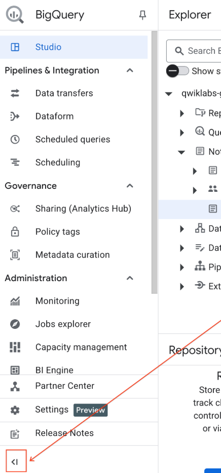
1. Google Cloud 콘솔에서 탐색 메뉴 > BigQuery로 이동합니다.

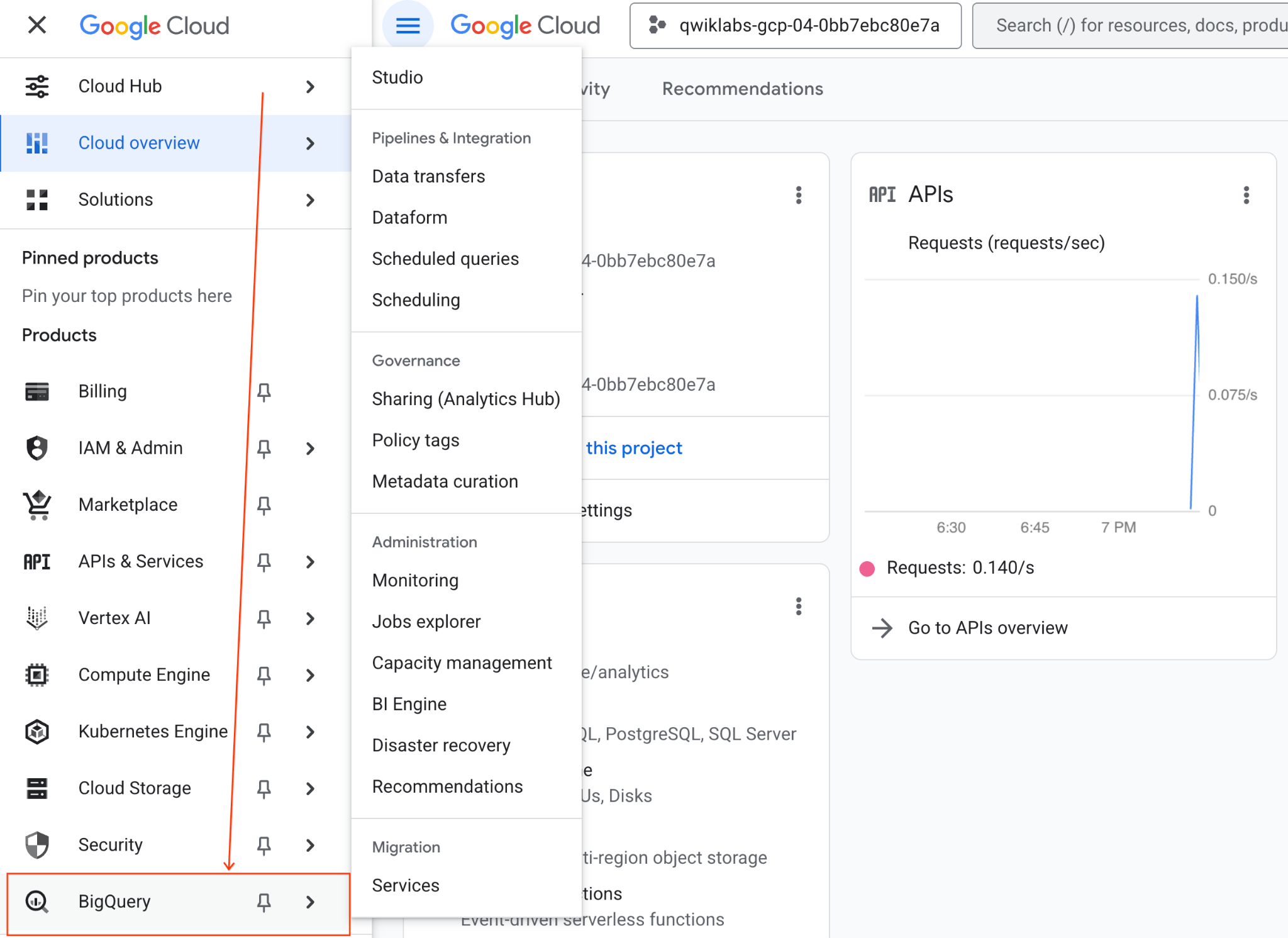
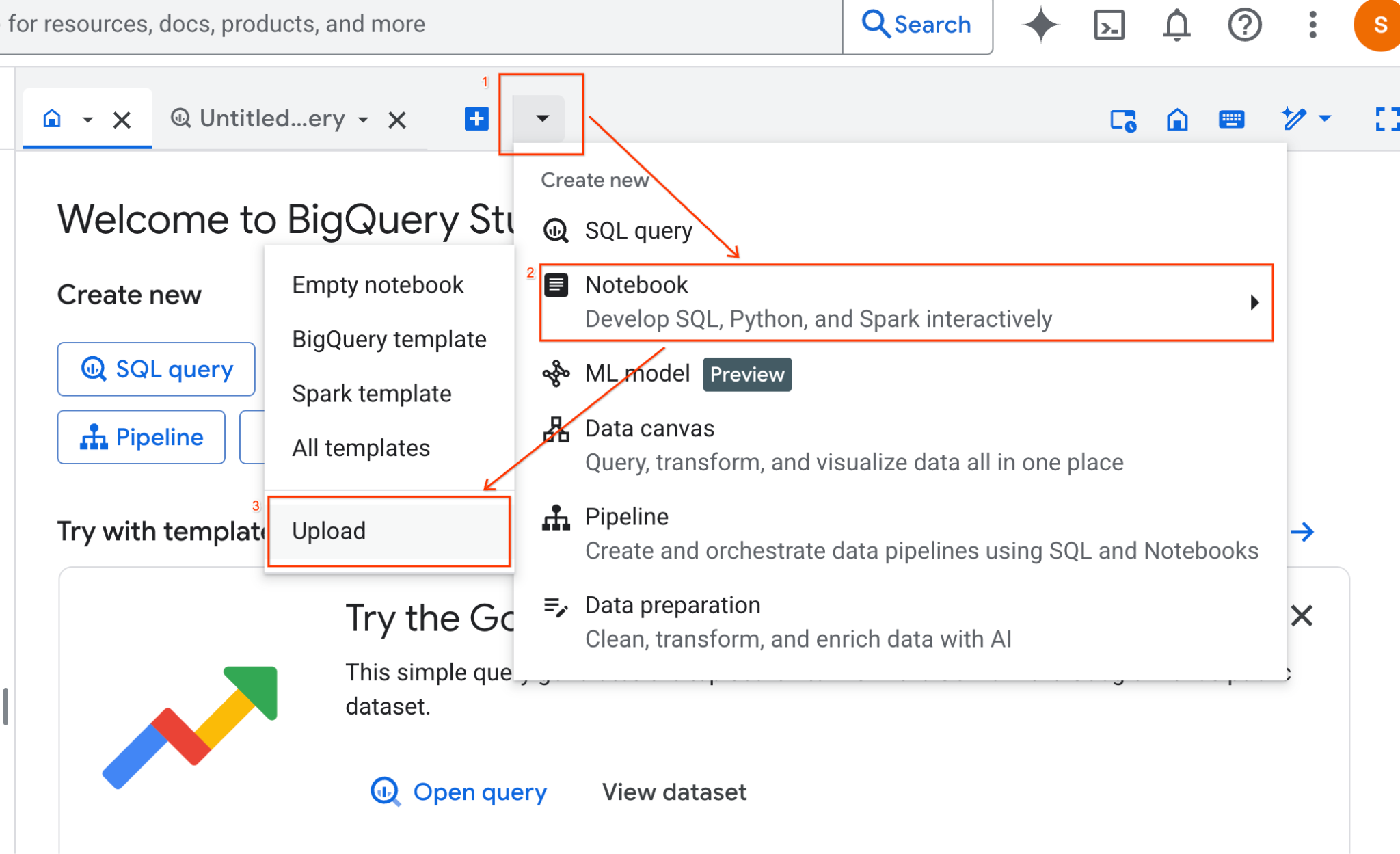
2. BigQuery Studio 창에서 드롭다운 화살표 버튼을 클릭하고 노트북 위로 마우스를 가져간 다음 업로드를 선택합니다.

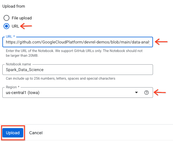
3. URL 라디오 버튼을 선택하고 다음 URL을 입력합니다.

https://github.com/GoogleCloudPlatform/devrel-demos/blob/main/data-analytics/dataproc-webinar/data-science/Spark_Data_Science.ipynb

4. 리전을 us-central11로 설정하고 업로드를 클릭합니다.

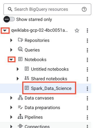
5. 노트북을 열려면 탐색기 창에서 프로젝트 ID 이름이 있는 드롭다운 화살표를 클릭합니다. 그런 다음 노트북 드롭다운을 클릭합니다. 노트북 Spark_Data_Science을 클릭합니다.

6. BigQuery 탐색 메뉴와 노트북의 목차를 접어 공간을 확보합니다.

3. 런타임에 연결하고 추가 설정 코드 실행

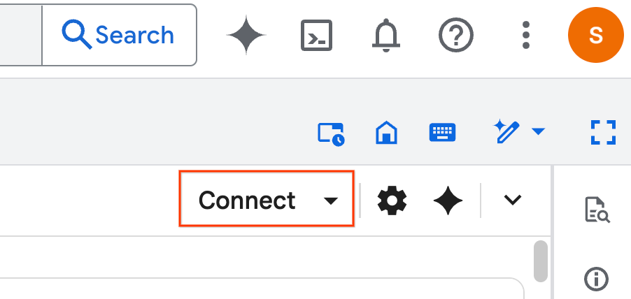
1. 연결을 클릭합니다. 팝업에서 이메일 계정으로 Colab Enterprise를 승인합니다. 노트북이 런타임에 자동으로 연결됩니다.

참고: 이 작업은 완료하는 데 몇 분 정도 걸릴 수 있습니다.

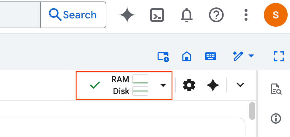
2. 런타임이 설정되면 다음이 표시됩니다.

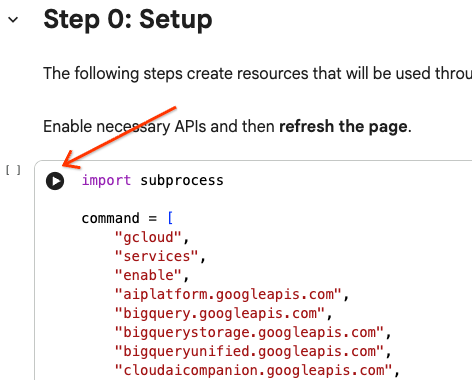
3. 노트북에서 설정 섹션으로 스크롤합니다. 여기에서 시작하세요.

참고: 노트북이 열리고 준비되면 이제 주로 Colab 환경 내에서 작업하게 됩니다. 이 노트북에는 전체 워크플로의 모든 코드와 자세한 셀별 설명이 포함되어 있습니다. 이 실습은 진행 상황을 추적하는 데 도움이 되는 간략한 요약을 제공하는 고급 가이드 역할을 합니다. 여기에서 Codelab 읽기를 중지해도 됩니다.

4. 설정 코드 실행

실습을 완료하는 데 필요한 Python 라이브러리로 환경을 구성합니다. 비공개 Google 액세스를 구성합니다. 스토리지 버킷을 만듭니다. BigQuery 데이터 세트를 만듭니다. 프로젝트 ID를 노트북에 복사합니다. 지역을 선택합니다. 이 실습에서는 us-central1 리전을 사용합니다.

셀 블록 안으로 커서를 가져간 다음 화살표를 클릭하여 코드 셀을 실행할 수 있습니다.

# Enable APIs
import subprocess

command = [
    "gcloud",
    "services",
    "enable",
    "aiplatform.googleapis.com",
    "bigquery.googleapis.com",
    "bigquerystorage.googleapis.com",
    "bigqueryunified.googleapis.com",
    "cloudaicompanion.googleapis.com",
    "dataproc.googleapis.com",
    "run.googleapis.com",
    "storage.googleapis.com"
]

result = subprocess.run(command, capture_output=True, text=True)
print(result.stdout)
print(result.stderr)

# Configure a PROJECT_ID and REGION
PROJECT_ID = "<YOUR_PROJECT_ID>"
REGION = "<YOUR_REGION>"

# Enable Private Google Access
import subprocess

command = [
    "gcloud",
    "compute",
    "networks",
    "subnets",
    "update",
    "default",
    f"--region={REGION}",
    "--enable-private-ip-google-access"
]

result = subprocess.run(command, capture_output=True, text=True)
print(result.stdout)
print(result.stderr)

# Create a Cloud Storage Bucket
from google.cloud import storage
from google.cloud.exceptions import NotFound

BUCKET_NAME = f"{PROJECT_ID}-demo"

storage_client = storage.Client(project=PROJECT_ID)
try:
    bucket = storage_client.get_bucket(BUCKET_NAME)
    print(f"Bucket {BUCKET_NAME} already exists.")
except NotFound:
    bucket = storage_client.create_bucket(BUCKET_NAME, location=REGION)
    print(f"Bucket {BUCKET_NAME} created.")


# Create a BigQuery dataset.
from google.cloud import bigquery

DATASET_ID = f"{PROJECT_ID}.demo"

client = bigquery.Client()

dataset = bigquery.Dataset(DATASET_ID)

dataset.location = REGION

dataset = client.create_dataset(dataset, exists_ok=True)

5. Apache Spark용 Google Cloud 서버리스에 대한 연결 만들기

Spark Connect를 사용하여 서버리스 Spark 세션에 연결하여 대화형 Spark 작업을 실행합니다. 고급 Spark 성능을 위해 Lightning Engine으로 런타임을 구성합니다. Lightning Engine은 Apache Gluten 및 Velox를 사용하여 워크로드를 가속화하는 방식으로 작동합니다.

from google.cloud.dataproc_spark_connect import DataprocSparkSession
from google.cloud.dataproc_v1 import Session

session = Session()

session.runtime_config.version = "3.0"

# You can optionally configure Spark properties as well. See https://cloud.google.com/dataproc-serverless/docs/concepts/properties.
session.runtime_config.properties = {
  "dataproc.runtime": "premium",
  "spark.dataproc.engine": "lightningEngine",
}

# To avoid going over quota in this demo, cap the max number of Spark workers.
session.runtime_config.properties = {
    "spark.dynamicAllocation.maxExecutors": "4"
}

spark = (
    DataprocSparkSession.builder
      .appName("CustomSparkSession")
      .dataprocSessionConfig(session)
      .getOrCreate()
)

6. Gemini를 사용하여 데이터 로드 및 탐색

이 섹션에서는 모든 데이터 과학 프로젝트의 첫 번째 중요한 단계인 데이터 준비를 살펴봅니다. 먼저 BigQuery에서 Apache Spark DataFrame으로 데이터를 로드합니다.

# Load the tables
order_items = spark.read.format("bigquery").option("table", "bigquery-public-data.thelook_ecommerce.order_items").load()

users = spark.read.format("bigquery").option("table", "bigquery-public-data.thelook_ecommerce.users").load()

# Register temp tables
users.createOrReplaceTempView("users")
order_items.createOrReplaceTempView("order_items")

# Verify temp tables
spark.sql("SELECT * FROM order_items LIMIT 10").show()

그런 다음 Gemini를 사용하여 PySpark 코드를 생성하여 데이터를 탐색하고 더 잘 이해합니다.

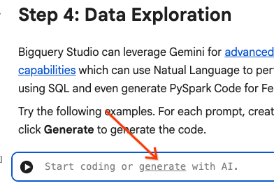
프롬프트 1: PySpark를 사용하여 users 테이블을 탐색하고 처음 10개 행을 표시해 줘.

# prompt:  Using PySpark, explore the users table and show the first 10 rows.

users.show(10)

프롬프트 2: PySpark를 사용하여 order_items 테이블을 살펴보고 처음 10개 행을 표시해 줘.

# prompt: Using PySpark, explore the order_items table and show the first 10 rows.

order_items.show(10)

프롬프트 3: PySpark를 사용하여 users 테이블에서 가장 빈도가 높은 상위 5개 국가를 표시해 줘. 국가와 각 국가의 사용자 수를 표시합니다.

# prompt: Using PySpark, show the top 5 most frequent countries in the users table. Display the country and the number of users from each country.

from pyspark.sql.functions import col, count

users.groupBy("country").agg(count("*").alias("user_count")).orderBy(col("user_count").desc()).limit(5).show()

프롬프트 4: PySpark를 사용하여 order_items 테이블에 있는 상품의 평균 판매 가격을 찾습니다.

# prompt: Using PySpark, find the average sale price of items in the order_items table.

from pyspark.sql import functions as F

average_sale_price = order_items.agg(F.avg("sale_price").alias("average_sale_price"))
average_sale_price.show()

프롬프트 5: 'users' 테이블을 사용하여 적절한 플로팅 라이브러리를 사용하여 국가와 트래픽 소스를 플롯하는 코드를 생성해 줘.

# prompt: Using the table "users", generate code to plot country vs traffic source using a suitable plotting library.

sql = """
    SELECT
        country,
        traffic_source
    FROM
        `bigquery-public-data.thelook_ecommerce.users`
    WHERE country IS NOT NULL AND traffic_source IS NOT NULL
"""
project_id = "iceberg-summit-2025"
df = pandas_gbq.read_gbq(sql, project_id=project_id, dialect="standard")

import matplotlib.pyplot as plt
import seaborn as sns

# Group by country and traffic_source and count occurrences
df_grouped = df.groupby(['country', 'traffic_source']).size().reset_index(name='count')

# Create a pivot table for easier plotting
pivot_table = df_grouped.pivot(index='country', columns='traffic_source', values='count').fillna(0)

# Plotting
plt.figure(figsize=(15, 8))
pivot_table.plot(kind='bar', stacked=True, figsize=(15, 8))
plt.title('Traffic Source Distribution by Country')
plt.xlabel('Country')
plt.ylabel('Number of Users')
plt.xticks(rotation=90)
plt.legend(title='Traffic Source')
plt.tight_layout()
plt.show()

프롬프트 6: '연령', '국가', '성별', 'traffic_source'의 분포를 보여주는 히스토그램을 만들어 줘.

# prompt: Create a histogram showing the distribution of "age", "country", "gender", "traffic_source".

import matplotlib.pyplot as plt

# Convert Spark DataFrame to Pandas DataFrame for visualization
users_pd = users.toPandas()

# Create histograms for 'age', 'country', 'gender', 'traffic_source'
fig, axes = plt.subplots(2, 2, figsize=(15, 10))
fig.suptitle('Distribution of User Attributes')

# Age distribution
axes[0, 0].hist(users_pd['age'].dropna(), bins=20, edgecolor='black')
axes[0, 0].set_title('Age Distribution')
axes[0, 0].set_xlabel('Age')
axes[0, 0].set_ylabel('Number of Users')

# Country distribution
users_pd['country'].value_counts().head(10).plot(kind='bar', ax=axes[0, 1])
axes[0, 1].set_title('Top 10 Countries Distribution')
axes[0, 1].set_xlabel('Country')
axes[0, 1].set_ylabel('Number of Users')
axes[0, 1].tick_params(axis='x', rotation=45)

# Gender distribution
users_pd['gender'].value_counts().plot(kind='bar', ax=axes[1, 0])
axes[1, 0].set_title('Gender Distribution')
axes[1, 0].set_xlabel('Gender')
axes[1, 0].set_ylabel('Number of Users')
axes[1, 0].tick_params(axis='x', rotation=0)

# Traffic Source distribution
users_pd['traffic_source'].value_counts().head(10).plot(kind='bar', ax=axes[1, 1])
axes[1, 1].set_title('Top 10 Traffic Source Distribution')
axes[1, 1].set_xlabel('Traffic Source')
axes[1, 1].set_ylabel('Number of Users')
axes[1, 1].tick_params(axis='x', rotation=45)

plt.tight_layout(rect=[0, 0.03, 1, 0.95])
plt.show()

7. 데이터 준비 및 특성 추출

다음으로 데이터에 특성 추출을 실행합니다. 적절한 열을 선택하고, 데이터를 더 적합한 데이터 유형으로 변환하고, 라벨 열을 식별합니다.

features = spark.sql("""
SELECT
  CAST(u.age AS DOUBLE) AS age,
  CAST(hash(u.country) AS BIGINT) * 1.0 AS country_hash,
  CAST(hash(u.gender) AS BIGINT) * 1.0 AS gender_hash,
  CAST(hash(u.traffic_source) AS BIGINT) * 1.0 AS traffic_source_hash,
  CASE WHEN COUNT(oi.id) > 0 THEN 1 ELSE 0 END AS label -- Changed label generation to count order items
FROM users AS u
LEFT JOIN order_items AS oi
ON u.id = oi.user_id
GROUP BY u.id, u.age, u.country, u.gender, u.traffic_source
""")
features.show()

8. 로지스틱 회귀 모델 학습

MLlib를 사용하여 로지스틱 회귀 모델을 학습시킵니다. 먼저 VectorAssembler을 사용하여 데이터를 벡터 형식으로 변환합니다. 그런 다음 StandardScaler에서 성능 향상을 위해 특징 열을 확장합니다. 그런 다음 LogisticRegression 모델에 대한 참조를 만들고 하이퍼파라미터를 정의합니다. 이러한 단계를 Pipeline 객체로 결합하고 fit() 함수를 사용하여 모델을 학습시키고 transform() 함수를 사용하여 데이터를 변환합니다.

from pyspark.ml.classification import LogisticRegression, LogisticRegressionModel
from pyspark.ml.evaluation import BinaryClassificationEvaluator
from pyspark.ml.feature import VectorAssembler, StandardScaler
from pyspark.ml.pipeline import Pipeline
from pyspark.ml.functions import array_to_vector

#Split Train and Test Data (80:20)
train_data, test_data = features.randomSplit([0.8, 0.2], seed=42)

# Initialize VectorAssembler
assembler = VectorAssembler(
    inputCols=["age", "country_hash", "gender_hash", "traffic_source_hash"],
    outputCol="assembled_features"
)

# Initialize StandardScaler
scaler = StandardScaler(inputCol="assembled_features", outputCol="scaled_features")

# Initialize Logistic Regression model
lr = LogisticRegression(
    maxIter=100,
    regParam=0.2,
    threshold=0.8,
    featuresCol="scaled_features",
    labelCol="label"
)

# Define pipeline
pipeline = Pipeline(stages=[assembler, scaler, lr])

# Fit the model
pipeline_model = pipeline.fit(train_data)

# Transform the dataset using the trained model
transformed_dataset = pipeline_model.transform(test_data)
transformed_dataset.show()

9. 모델 평가

새로 변환된 데이터 세트를 평가합니다. 평가 측정항목 곡선 아래 영역 (AUC)을 생성합니다.

# Model evaluation
eva = BinaryClassificationEvaluator(metricName="areaUnderPR")
aucPR = eva.evaluate(transformed_dataset)
print(f"AUC PR: {aucPR}")

그런 다음 Gemini를 사용하여 모델 출력을 시각화하는 PySpark 코드를 생성합니다.

프롬프트 1: 정밀도-재현율 (PR) 곡선을 그리는 코드를 생성해 줘. 모델의 예측에서 정밀도와 재현율을 계산하고 적절한 플로팅 라이브러리를 사용하여 PR 곡선을 표시합니다.

# prompt: Generate code to plot the Precision-Recall (PR) curve. Calculate precision and recall from the model's predictions and display the PR curve using a suitable plotting library.

import matplotlib.pyplot as plt
from sklearn.metrics import precision_recall_curve, auc

# Extract predictions and labels
predictions = transformed_dataset.select("prediction", "label").toPandas()

# Calculate precision and recall
precision, recall, _ = precision_recall_curve(predictions["label"], predictions["prediction"])

# Calculate AUC-PR
pr_auc = auc(recall, precision)

# Plot the PR curve
plt.figure(figsize=(8, 6))
plt.plot(recall, precision, color='blue', lw=2, label=f'PR curve (AUC = {pr_auc:.2f})')
plt.xlabel('Recall')
plt.ylabel('Precision')
plt.title('Precision-Recall Curve')
plt.legend(loc='lower left')
plt.grid(True)
plt.show()

프롬프트 2: 혼동 행렬 시각화를 만드는 코드를 생성해 줘. 모델의 예측에서 혼동 행렬을 계산하고 참양성 (TP), 참음성 (TN), 거짓양성 (FP), 거짓음성 (FN)의 개수가 포함된 히트맵 또는 표로 표시합니다.

# prompt: Generate code to create a confusion matrix visualization. Calculate the confusion matrix from the model's predictions and display it as a heat map or a table with counts of true positives (TP), true negatives (TN), false positives (FP), and false negatives (FN).

import pandas as pd
import seaborn as sns
import matplotlib.pyplot as plt
from sklearn.metrics import confusion_matrix

# Extract predictions and labels
predictions_and_labels = transformed_dataset.select("prediction", "label").toPandas()

# Calculate the confusion matrix
cm = confusion_matrix(predictions_and_labels["label"], predictions_and_labels["prediction"])

# Create a DataFrame for better visualization
cm_df = pd.DataFrame(cm,
                     index=['Actual Negative', 'Actual Positive'],
                     columns=['Predicted Negative', 'Predicted Positive'])

# Display the confusion matrix as a table
print("Confusion Matrix:")
print(cm_df)

# Display the confusion matrix as a heatmap
plt.figure(figsize=(8, 6))
sns.heatmap(cm_df, annot=True, fmt='d', cmap='Blues', cbar=False, linewidths=.5)
plt.title('Confusion Matrix')
plt.ylabel('Actual Label')
plt.xlabel('Predicted Label')
plt.show()

# Calculate and display TP, TN, FP, FN
TN, FP, FN, TP = cm.ravel()
print(f"
True Positives (TP): {TP}")
print(f"True Negatives (TN): {TN}")
print(f"False Positives (FP): {FP}")
print(f"False Negatives (FN): {FN}")

10. BigQuery에 예측 쓰기

Gemini를 사용하여 BigQuery 데이터 세트의 새 테이블에 예측을 작성하는 코드를 생성합니다.

프롬프트: Spark를 사용하여 변환된 데이터 세트를 BigQuery에 작성해 줘.

# prompt: Using Spark, write the transformed dataset to BigQuery.

transformed_dataset.write.format("bigquery").option("table", f"{PROJECT_ID}.demo.predictions").mode("overwrite").save()

11. Cloud Storage에 모델 저장

MLlib의 기본 기능을 사용하여 모델을 Cloud Storage에 저장합니다. 추론 서버는 여기에서 모델을 로드합니다.

MODEL_PATH = "models/prediction_model"
pipeline_model.write().overwrite().save(f"gs://{BUCKET_NAME}/{MODEL_PATH}")

12. 추론 서버 만들기

Cloud Run은 서버리스 웹 앱을 실행하는 유연한 도구입니다. Docker 컨테이너를 사용하여 사용자에게 최대한의 맞춤설정 기능을 제공합니다. 이 실습에서는 PySpark를 지원하는 Flask 앱을 실행하도록 Dockerfile이 구성되어 있습니다. 이 컨테이너는 Cloud Run에서 실행되어 입력 데이터에 대한 추론을 실행합니다. 이 코드는 여기에서 확인할 수 있습니다.

추론 서버 코드로 저장소를 클론합니다.

!git clone https://github.com/GoogleCloudPlatform/devrel-demos.git

Dockerfile을 확인합니다.

FROM python:3.12-slim

# Install OpenJDK-21 (Required for Spark)
RUN apt-get update && \
    apt-get install -y openjdk-21-jre-headless procps && \
    rm -rf /var/lib/apt/lists/*

ENV JAVA_HOME=/usr/lib/jvm/java-21-openjdk-amd64
ENV PORT=8080

WORKDIR /app

COPY requirements.txt .
RUN pip install --no-cache-dir -r requirements.txt

COPY main.py .

CMD ["gunicorn", "--bind", "0.0.0.0:8080", "--workers", "1", "--threads", "8", "--timeout", "0", "main:app"]

서버의 Python 코드를 확인합니다.

import os
import json
import logging

from flask import Flask, request, jsonify
from google.cloud import storage
from pyspark.ml import PipelineModel
from pyspark.sql import SparkSession
from pyspark.sql.functions import hash, col

# Configure basic logging
logging.basicConfig(level=logging.INFO, format='%(asctime)s - %(levelname)s - %(message)s')

# --- Initialization: Spark and Model Loading ---
GCS_BUCKET = os.environ.get("GCS_BUCKET")
GCS_MODEL_PATH = os.environ.get("GCS_MODEL_PATH")
LOCAL_MODEL_PATH = "/tmp/model"

try:
    spark = SparkSession.builder \
        .appName("CloudRunSparkService") \
        .master("local[*]") \
        .getOrCreate()
    logging.info("Spark Session successfully initialized.")
except Exception as e:
    logging.error(f"Failed to initialize Spark Session: {e}")
    raise

def download_directory(bucket_name, prefix, local_path):
    """Downloads a directory from GCS to local filesystem."""
    storage_client = storage.Client()
    bucket = storage_client.get_bucket(bucket_name)
    blobs = list(bucket.list_blobs(prefix=prefix))
    
    if len(blobs) == 0:
        logging.error(f"No files found in GCS bucket {bucket_name} at prefix {prefix}")
        return
    
    for blob in blobs:
        if blob.name.endswith("/"): continue # Skip directories
        
        # Structure local paths
        relative_path = os.path.relpath(blob.name, prefix)
        local_file_path = os.path.join(local_path, relative_path)
        os.makedirs(os.path.dirname(local_file_path), exist_ok=True)
        
        blob.download_to_filename(local_file_path)
    print(f"Model downloaded to {local_path}")

# Load model
def load_model(LOCAL_MODEL_PATH, GCS_BUCKET, GCS_MODEL_PATH):
    """Download and load model on startup to avoid latency per request."""
    global MODEL
    if not os.path.exists(LOCAL_MODEL_PATH):
        download_directory(GCS_BUCKET, GCS_MODEL_PATH, LOCAL_MODEL_PATH)
    
    logging.info(f"Loading PySpark model from {GCS_MODEL_PATH}")
    # Load the Spark ML model
    try:
        MODEL = PipelineModel.load(LOCAL_MODEL_PATH)
        logging.info("Spark model loaded successfully.")
    except Exception as e:
        logging.error(f"Failed to load model: {e}")
        raise
    
# Load Model on Startup
load_model(LOCAL_MODEL_PATH, GCS_BUCKET, GCS_MODEL_PATH)

# --- Flask Application Setup ---
app = Flask(__name__)

@app.route('/predict', methods=['POST'])
def predict():
    """
    Handles incoming POST requests for inference.
    Expects JSON data that can be converted into a Spark DataFrame.
    """
    if MODEL is None:
        return jsonify({"error": "Model failed to load at startup."}), 500

    try:
        # 1. Get data from the request
        data = request.get_json()
        
        # 2. Check length of list
        data_len = len(data)
        cap = 100
        if data_len > cap:
            return jsonify({"error": f"Too many records. Count: {data_len}, Max: {cap}"}), 400

        # 2. Create Spark DataFrame
        df = spark.createDataFrame(data)
        
        # 3. Transform data
        input_df = df.select(
            col("age").cast("DOUBLE").alias("age"), 
            (hash(col("country")).cast("BIGINT") * 1.0).alias("country_hash"),
            (hash(col("gender")).cast("BIGINT") * 1.0).alias("gender_hash"),
            (hash(col("traffic_source")).cast("BIGINT") * 1.0).alias("traffic_source_hash")
        )

        # 3. Perform Inference
        predictions_df = MODEL.transform(input_df)

        # 4. Prepare results (collect and serialize)
        results = [p.prediction for p in predictions_df.select("prediction").collect()]

        # 5. Return JSON response
        return jsonify({"predictions": results})

    except Exception as e:
        logging.error(f"An error occurred during prediction: {e}")
        #return jsonify({"error": str(e)}), 500
        raise e  
    
# Gunicorn entry point uses 'app' from this file
if __name__ == '__main__':
    # Local testing only: Cloud Run uses Gunicorn/CMD command
    app.run(host='0.0.0.0', port=int(os.environ.get('PORT', 8080)))

추론 서버를 배포합니다.

import subprocess

command = [
    "gcloud",
    "run",
    "deploy",
    "inference-server",
    "--source",
    "/content/devrel-demos/data-analytics/dataproc-webinar/data-science/inference-server",
    "--region",
    f"{REGION}",
    "--port",
    "8080",
    "--memory",
    "2Gi",
    "--allow-unauthenticated",
    "--set-env-vars",
    f"GCS_BUCKET={BUCKET_NAME},GCS_MODEL_PATH={MODEL_PATH}",
    "--startup-probe",
    "tcpSocket.port=8080,initialDelaySeconds=240,failureThreshold=3,timeoutSeconds=240,periodSeconds=240"
]

result = subprocess.run(command, capture_output=True, text=True)
print(result.stdout)
print(result.stderr)

출력에서 추론 서버 URL을 새 변수로 복사합니다. https://inference-server-123456789.us-central1.run.app.와 유사합니다.

INFERENCE_SERVER_URL = "<YOUR_SERVER_URL>"

추론 서버를 테스트합니다.

import requests

age = "25.0"
country = "United States"
traffic_source = "Search"
gender = "F"

response = requests.post(
    f"{INFERENCE_SERVER_URL}/predict",
    json=[{"age": age, "country": country, "traffic_source": traffic_source, "gender": gender}],
    headers={"Content-Type": "application/json"}
)

print(response.json())

출력은 1.0 또는 0.0이어야 합니다.

{'predictions': [1.0]}

13. 에이전트 구성

Agent Engine을 사용하여 추론을 실행할 수 있는 에이전트를 만듭니다. Agent Engine은 개발자가 프로덕션에서 AI 에이전트를 배포, 관리, 확장할 수 있도록 지원하는 서비스 모음인 Vertex AI Platform의 일부입니다. 여기에는 에이전트, 세션 컨텍스트, 코드 실행을 평가하는 등 다양한 도구가 있습니다. 에이전트 개발 키트 (ADK)를 비롯한 다양한 인기 에이전트 프레임워크를 지원합니다. ADK는 Gemini 및 Google 생태계와의 사용을 위해 빌드되고 최적화되었지만 모델에 구애받지 않는 오픈소스 에이전트 프레임워크입니다. 에이전트 개발이 소프트웨어 개발과 유사하게 느껴지도록 설계되었습니다.

Vertex AI 클라이언트를 초기화합니다.

import vertexai
from vertexai import agent_engines # For the prebuilt templates

client = vertexai.Client(  # For service interactions via client.agent_engines
    project=f"{PROJECT_ID}",
    location=f"{REGION}",
)

배포된 모델을 쿼리하는 함수를 정의합니다.

def predict_purchase(
    age: str = "25.0",
    country: str = "United States",
    traffic_source: str = "Search",
    gender: str = "M",
):
    """Predicts whether or not a user will purchase a product.

    Args:
        age: The age of the user.
        country: The country of the user. One of: "China", "Poland", "Germany", "United States", "Spain", "United Kingdom", "España", "Japan", "Brasil", "Colombia", "Belgium", "South Korea", "Austria", "France", "Australia".
        Traffic_source: The source of the user's traffic. One of: "Display", "Email", "Search", "Organic", "Facebook".
        gender: The gender of the user. One of: "M" or "F".

    Returns:
        True if the model output is 1.0, False otherwise.
    """
    import requests
    response = requests.post(
        f"{INFERENCE_SERVER_URL}/predict",
        json=[{"age": age, "country": country, "traffic_source": traffic_source, "gender": gender}],
        headers={"Content-Type": "application/json"}
    )
    return response.json()

샘플 매개변수를 전달하여 함수를 테스트합니다.

predict_purchase(age=25.0, country="United States", traffic_source="Search", gender="M")

ADK를 사용하여 아래에 에이전트를 정의하고 predict_purchase 함수를 도구로 제공합니다.

from google.adk.agents import Agent
from vertexai import agent_engines

agent = Agent(
   model="gemini-2.5-flash",
   name='purchase_prediction_agent',
   tools=[predict_purchase]
)

쿼리를 전달하여 로컬로 에이전트를 테스트합니다.

app = agent_engines.AdkApp(agent=agent)
async for event in app.async_stream_query(
    user_id="123",
    message="Will a 25 yo male from the United States who came from Search make a purchase? Strictly output 'yes' or 'no'.",
):
    try:
        print(event['content']['parts'][0]['text'])
    except:
      continue

모델을 Agent Engine에 배포합니다.

remote_agent = client.agent_engines.create(
    agent=app,
    config={
        "requirements": ["google-cloud-aiplatform[agent_engines,adk]"],
        "staging_bucket": f"gs://{BUCKET_NAME}",
        "display_name": "purchase-predictor",
        "description": "Agent that predicts whether or not a user will purchase a product.",
    }
)

완료되면 Cloud 콘솔에서 배포된 모델을 확인합니다.

모델을 다시 쿼리합니다. 이제 로컬 버전이 아닌 배포된 에이전트를 가리킵니다.

async for event in remote_agent.async_stream_query(
    user_id="123",
    message="Will a 25 yo male from the United States who came from Search make a purchase? Strictly output 'yes' or 'no'.",
):
    try:
        print(event['content']['parts'][0]['text'])
    except:
      continue

14. 삭제

생성한 모든 Google Cloud 리소스를 삭제합니다. 이와 같은 정리 명령어를 실행하는 것은 향후 요금이 청구되지 않도록 하는 데 중요한 권장사항입니다.

# Delete the deployed agent.
remote_agent.delete(force=True)

# Delete the inference server.
import subprocess

command = [
    "gcloud",
    "run",
    "services",
    "delete",
    "inference-server",
    "--region",
    f"{REGION}",
    "--quiet"
]

subprocess.run(command, capture_output=True, text=True)

# Delete the BigQuery dataset.
bigquery_client = bigquery.Client()

bigquery_client.delete_dataset(
    f"{PROJECT_ID}.demo", delete_contents=True, not_found_ok=True
)

# Delete the Storage bucket.
storage_client = storage.Client()

bucket = storage_client.get_bucket(BUCKET_NAME)
bucket.delete_blobs(list(bucket.list_blobs()))
bucket.delete()

15. 축하합니다.

축하드립니다. 이 Codelab에서는 다음 작업을 수행했습니다.

• BigQuery Studio 노트북을 사용하여 데이터 과학 워크플로를 실행했습니다.
• Apache Spark용 Google Cloud 서버리스를 사용하여 Apache Spark에 연결을 만들고 Spark Connect로 구동됩니다.
• Lightning Engine을 사용하여 Apache Spark 워크로드를 최대 4.3배 가속화했습니다.
• Apache Spark와 BigQuery 간의 기본 제공 통합을 사용하여 BigQuery에서 데이터를 로드했습니다.
• Gemini 지원 코드 생성을 사용하여 데이터를 탐색했습니다.
• Apache Spark의 데이터 처리 프레임워크를 사용하여 특성 엔지니어링을 실행했습니다.
• Apache Spark의 기본 머신러닝 라이브러리인 MLlib를 사용하여 분류 모델을 학습시키고 평가했습니다.
• Flask 및 Cloud Run을 사용하여 분류 모델의 추론 서버를 배포했습니다.
• Agent Engine 및 에이전트 개발 키트 (ADK)를 사용하여 자연어로 추론 서버를 쿼리하는 에이전트를 배포했습니다.

다음 단계

• Apache Spark용 Google Cloud 서버리스에 대해 자세히 알아보세요.
• Cloud Run을 구성하는 방법을 알아보세요.
• Agent Engine에 대해 읽어봅니다.