Spark ile Veri Bilimi

1. Genel Bakış

Varsayımsal bir e-ticaret giyim perakendecisi olan TheLook, müşteriler, ürünler, siparişler, lojistik, web etkinlikleri ve dijital pazarlama kampanyalarıyla ilgili verileri BigQuery'de saklar. Şirket, Apache Spark kullanarak bu verileri analiz etmek için ekibin mevcut SQL ve PySpark uzmanlığından yararlanmak istiyor.

TheLook, Spark için manuel altyapı sağlama veya ince ayar yapma işlemlerinden kaçınmak amacıyla küme yönetimi yerine iş yüklerine odaklanmalarını sağlayacak bir otomatik ölçeklendirme çözümü arıyor. Ayrıca, BigQuery Studio ortamında kalırken Spark ve BigQuery'yi entegre etmek için gereken çabayı en aza indirmek istiyorlar.

Bu laboratuvarda, PySpark kullanarak bir lojistik regresyon sınıflandırıcı oluşturacak ve verileri keşfetmek için BigQuery Studio'nun yerel not defteri entegrasyonundan ve yapay zeka özelliklerinden yararlanarak bir kullanıcının satın alma işlemi yapıp yapmayacağını tahmin edeceksiniz. Bu modeli bir çıkarım sunucusuna dağıtır ve modeli doğal dil kullanarak sorgulamak için bir aracı oluşturursunuz.

Ön koşullar

Bu laboratuvara başlamadan önce şunlar hakkında bilgi sahibi olmanız gerekir:

Temel SQL ve Python programlama
Jupyter not defterinde Python kodu çalıştırma
Dağıtılmış bilgi işlem hakkında temel düzeyde bilgi sahibi olma

Hedefler

Veri bilimi iş akışı çalıştırmak için BigQuery Studio not defterlerini kullanın.
Google Cloud Serverless for Apache Spark'ı kullanarak ve Spark Connect ile desteklenen Apache Spark bağlantısı oluşturun.
Apache Spark iş yüklerini 4,3 kata kadar hızlandırmak için Lightning Engine'i kullanın.
Apache Spark ile BigQuery arasındaki yerleşik entegrasyonu kullanarak BigQuery'den veri yükleyin.
Gemini destekli kod oluşturma özelliğini kullanarak verileri keşfedin.
Apache Spark'ın veri işleme çerçevesini kullanarak özellik mühendisliği yapın.
Apache Spark'ın yerel makine öğrenimi kitaplığı MLlib'i kullanarak bir sınıflandırma modelini eğitme ve değerlendirme
Flask ve Cloud Run kullanarak sınıflandırma modeli için çıkarım sunucusu dağıtma
Agent Engine ve Agent Development Kit (ADK) ile çıkarım sunucusunu doğal dilde sorgulamak için bir temsilci dağıtma,

2. Colab çalışma zamanı ortamına bağlanma

Google Cloud projesi belirleme

Google Cloud projesi oluşturun. Mevcut bir hesabı kullanabilirsiniz.

Önerilen API'leri etkinleştirme:

Aşağıdaki API'leri etkinleştirmek için burayı tıklayın:

Kullanıcı arayüzünde gezinme:

Google Cloud Console'da Gezinme menüsü > BigQuery'ye gidin.

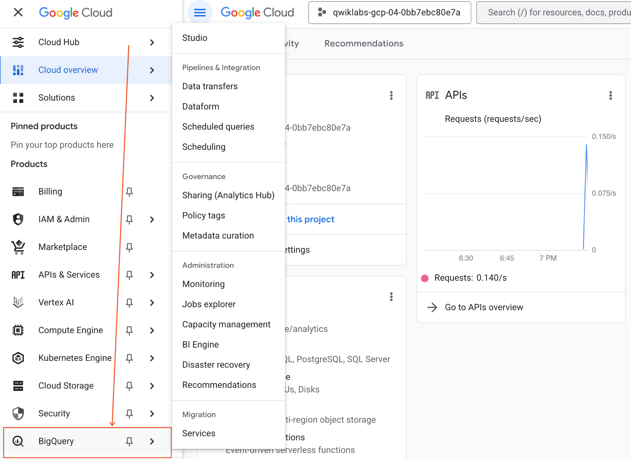
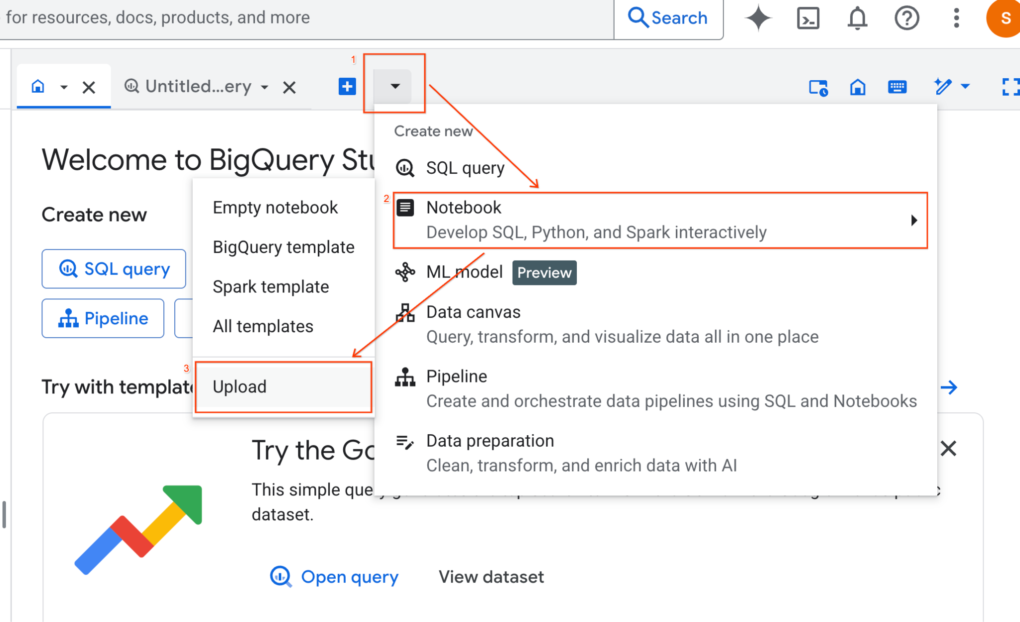
Google Cloud Console'daki BigQuery sekmesini gösteren bir ok.

BigQuery Studio bölmesinde açılır liste oku düğmesini tıklayın, fareyle Not Defteri'nin üzerine gelin ve Yükle'yi seçin.

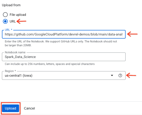
URL radyo düğmesini seçin ve aşağıdaki URL'yi girin:

https://github.com/GoogleCloudPlatform/devrel-demos/blob/main/data-analytics/dataproc-webinar/data-science/Spark_Data_Science.ipynb

Bölgeyi us-central11 olarak ayarlayın ve Yükle'yi tıklayın.

Not defterini açmak için Gezgin bölmesinde proje kimliğinizin adını içeren açılır liste okunuzu tıklayın. Ardından Not Defterleri açılır menüsünü tıklayın. Not defterini Spark_Data_Science tıklayın.

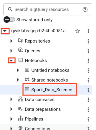
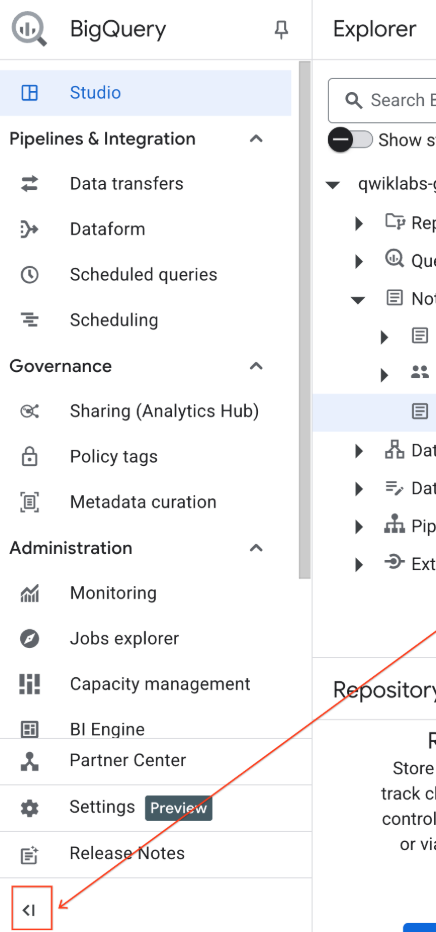
Daha fazla alan için BigQuery gezinme menüsünü ve not defterinin içindekiler tablosunu daraltın.

3. Çalışma zamanına bağlanma ve ek kurulum kodu çalıştırma

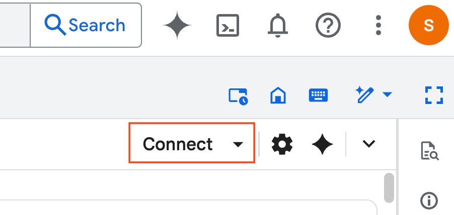
Bağlan'ı tıklayın. Pop-up pencerede, e-posta hesabınızla Colab Enterprise'ı yetkilendirin. Not defteriniz otomatik olarak bir çalışma zamanına bağlanır.

Çalışma zamanı belirlendikten sonra aşağıdakileri görürsünüz:

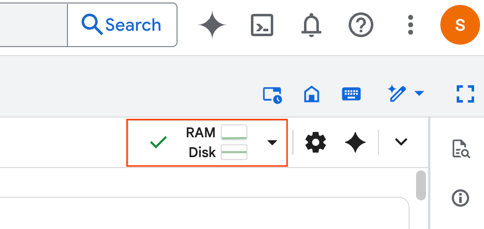
Not defterinde Kurulum bölümüne gidin. Buradan başlayın.

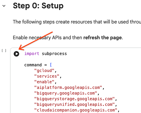
4. Kurulum kodunu çalıştırma

Laboratuvarı tamamlamak için ortamınızı gerekli Python kitaplıklarıyla yapılandırın. Özel Google Erişimi'ni yapılandırın. Storage paketi oluşturun. Bir BigQuery veri kümesi oluşturun. Proje kimliğinizi not defterine kopyalayın. Bir bölge seçin. Bu laboratuvarda us-central1 bölgesini kullanın.

İmlecinizi hücre bloğunun içine getirip oku tıklayarak kod hücresini çalıştırabilirsiniz.

# Enable APIs
import subprocess

command = [
    "gcloud",
    "services",
    "enable",
    "aiplatform.googleapis.com",
    "bigquery.googleapis.com",
    "bigquerystorage.googleapis.com",
    "bigqueryunified.googleapis.com",
    "cloudaicompanion.googleapis.com",
    "dataproc.googleapis.com",
    "run.googleapis.com",
    "storage.googleapis.com"
]

result = subprocess.run(command, capture_output=True, text=True)
print(result.stdout)
print(result.stderr)

# Configure a PROJECT_ID and REGION
PROJECT_ID = "<YOUR_PROJECT_ID>"
REGION = "<YOUR_REGION>"

# Enable Private Google Access
import subprocess

command = [
    "gcloud",
    "compute",
    "networks",
    "subnets",
    "update",
    "default",
    f"--region={REGION}",
    "--enable-private-ip-google-access"
]

result = subprocess.run(command, capture_output=True, text=True)
print(result.stdout)
print(result.stderr)

# Create a Cloud Storage Bucket
from google.cloud import storage
from google.cloud.exceptions import NotFound

BUCKET_NAME = f"{PROJECT_ID}-demo"

storage_client = storage.Client(project=PROJECT_ID)
try:
    bucket = storage_client.get_bucket(BUCKET_NAME)
    print(f"Bucket {BUCKET_NAME} already exists.")
except NotFound:
    bucket = storage_client.create_bucket(BUCKET_NAME, location=REGION)
    print(f"Bucket {BUCKET_NAME} created.")


# Create a BigQuery dataset.
from google.cloud import bigquery

DATASET_ID = f"{PROJECT_ID}.demo"

client = bigquery.Client()

dataset = bigquery.Dataset(DATASET_ID)

dataset.location = REGION

dataset = client.create_dataset(dataset, exists_ok=True)

5. Google Cloud Serverless for Apache Spark ile bağlantı oluşturma

Spark Connect'i kullanarak etkileşimli Spark işlerini çalıştırmak için sunucusuz bir Spark oturumuna bağlanırsınız. Gelişmiş Spark performansı için çalışma zamanınızı Lightning Engine ile yapılandırın. Lightning Engine, Apache Gluten ve Velox kullanarak iş yüklerini hızlandırır.

from google.cloud.dataproc_spark_connect import DataprocSparkSession
from google.cloud.dataproc_v1 import Session

session = Session()

session.runtime_config.version = "3.0"

# You can optionally configure Spark properties as well. See https://cloud.google.com/dataproc-serverless/docs/concepts/properties.
session.runtime_config.properties = {
  "dataproc.runtime": "premium",
  "spark.dataproc.engine": "lightningEngine",
}

# To avoid going over quota in this demo, cap the max number of Spark workers.
session.runtime_config.properties = {
    "spark.dynamicAllocation.maxExecutors": "4"
}

spark = (
    DataprocSparkSession.builder
      .appName("CustomSparkSession")
      .dataprocSessionConfig(session)
      .getOrCreate()
)

6. Gemini'ı kullanarak verileri yükleme ve keşfetme

Bu bölümde, herhangi bir veri bilimi projesindeki ilk önemli adım olan verilerinizi hazırlama sürecini ele alacağız. Öncelikle BigQuery'den Apache Spark veri çerçevesine veri yükleyerek başlarsınız.

# Load the tables
order_items = spark.read.format("bigquery").option("table", "bigquery-public-data.thelook_ecommerce.order_items").load()

users = spark.read.format("bigquery").option("table", "bigquery-public-data.thelook_ecommerce.users").load()

# Register temp tables
users.createOrReplaceTempView("users")
order_items.createOrReplaceTempView("order_items")

# Verify temp tables
spark.sql("SELECT * FROM order_items LIMIT 10").show()

Ardından, verileri keşfetmek ve daha iyi anlamak için PySpark kodu oluşturmak üzere Gemini'ı kullanırsınız.

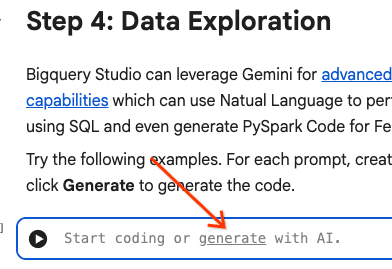
İstem 1: PySpark'ı kullanarak kullanıcılar tablosunu keşfedin ve ilk 10 satırı gösterin.

# prompt:  Using PySpark, explore the users table and show the first 10 rows.

users.show(10)

2. istem: PySpark'ı kullanarak order_items tablosunu keşfedin ve ilk 10 satırı gösterin.

# prompt: Using PySpark, explore the order_items table and show the first 10 rows.

order_items.show(10)

3. istem: PySpark'ı kullanarak kullanıcılar tablosundaki en sık kullanılan 5 ülkeyi göster. Ülkeyi ve her ülkeden gelen kullanıcı sayısını gösterin.

# prompt: Using PySpark, show the top 5 most frequent countries in the users table. Display the country and the number of users from each country.

from pyspark.sql.functions import col, count

users.groupBy("country").agg(count("*").alias("user_count")).orderBy(col("user_count").desc()).limit(5).show()

4. istem: PySpark'ı kullanarak order_items tablosundaki öğelerin ortalama indirimli fiyatını bulun.

# prompt: Using PySpark, find the average sale price of items in the order_items table.

from pyspark.sql import functions as F

average_sale_price = order_items.agg(F.avg("sale_price").alias("average_sale_price"))
average_sale_price.show()

5. istem: "Kullanıcılar" tablosunu kullanarak uygun bir çizim kitaplığıyla ülke ve trafik kaynağına göre çizim yapacak kodu oluşturun.

# prompt: Using the table "users", generate code to plot country vs traffic source using a suitable plotting library.

sql = """
    SELECT
        country,
        traffic_source
    FROM
        `bigquery-public-data.thelook_ecommerce.users`
    WHERE country IS NOT NULL AND traffic_source IS NOT NULL
"""
project_id = "iceberg-summit-2025"
df = pandas_gbq.read_gbq(sql, project_id=project_id, dialect="standard")

import matplotlib.pyplot as plt
import seaborn as sns

# Group by country and traffic_source and count occurrences
df_grouped = df.groupby(['country', 'traffic_source']).size().reset_index(name='count')

# Create a pivot table for easier plotting
pivot_table = df_grouped.pivot(index='country', columns='traffic_source', values='count').fillna(0)

# Plotting
plt.figure(figsize=(15, 8))
pivot_table.plot(kind='bar', stacked=True, figsize=(15, 8))
plt.title('Traffic Source Distribution by Country')
plt.xlabel('Country')
plt.ylabel('Number of Users')
plt.xticks(rotation=90)
plt.legend(title='Traffic Source')
plt.tight_layout()
plt.show()

6. istem: "Yaş", "ülke", "cinsiyet", "traffic_source" dağılımını gösteren bir histogram oluştur.

# prompt: Create a histogram showing the distribution of "age", "country", "gender", "traffic_source".

import matplotlib.pyplot as plt

# Convert Spark DataFrame to Pandas DataFrame for visualization
users_pd = users.toPandas()

# Create histograms for 'age', 'country', 'gender', 'traffic_source'
fig, axes = plt.subplots(2, 2, figsize=(15, 10))
fig.suptitle('Distribution of User Attributes')

# Age distribution
axes[0, 0].hist(users_pd['age'].dropna(), bins=20, edgecolor='black')
axes[0, 0].set_title('Age Distribution')
axes[0, 0].set_xlabel('Age')
axes[0, 0].set_ylabel('Number of Users')

# Country distribution
users_pd['country'].value_counts().head(10).plot(kind='bar', ax=axes[0, 1])
axes[0, 1].set_title('Top 10 Countries Distribution')
axes[0, 1].set_xlabel('Country')
axes[0, 1].set_ylabel('Number of Users')
axes[0, 1].tick_params(axis='x', rotation=45)

# Gender distribution
users_pd['gender'].value_counts().plot(kind='bar', ax=axes[1, 0])
axes[1, 0].set_title('Gender Distribution')
axes[1, 0].set_xlabel('Gender')
axes[1, 0].set_ylabel('Number of Users')
axes[1, 0].tick_params(axis='x', rotation=0)

# Traffic Source distribution
users_pd['traffic_source'].value_counts().head(10).plot(kind='bar', ax=axes[1, 1])
axes[1, 1].set_title('Top 10 Traffic Source Distribution')
axes[1, 1].set_xlabel('Traffic Source')
axes[1, 1].set_ylabel('Number of Users')
axes[1, 1].tick_params(axis='x', rotation=45)

plt.tight_layout(rect=[0, 0.03, 1, 0.95])
plt.show()

7. Veri hazırlama ve özellik mühendisliği

Ardından, veriler üzerinde özellik mühendisliği yaparsınız. Uygun sütunları seçin, verileri daha uygun veri türlerine dönüştürün ve bir etiket sütunu belirleyin.

features = spark.sql("""
SELECT
  CAST(u.age AS DOUBLE) AS age,
  CAST(hash(u.country) AS BIGINT) * 1.0 AS country_hash,
  CAST(hash(u.gender) AS BIGINT) * 1.0 AS gender_hash,
  CAST(hash(u.traffic_source) AS BIGINT) * 1.0 AS traffic_source_hash,
  CASE WHEN COUNT(oi.id) > 0 THEN 1 ELSE 0 END AS label -- Changed label generation to count order items
FROM users AS u
LEFT JOIN order_items AS oi
ON u.id = oi.user_id
GROUP BY u.id, u.age, u.country, u.gender, u.traffic_source
""")
features.show()

8. Mantıksal regresyon modeli eğitme

MLlib'i kullanarak bir mantıksal regresyon modeli eğitirsiniz. Öncelikle verileri vektör biçimine dönüştürmek için VectorAssembler kullanırsınız. Ardından, StandardScaler daha iyi performans için özellikler sütununu ölçeklendirir. Ardından, LogisticRegression modeline referans oluşturup hiperparametreleri tanımlarsınız. Bu adımları bir Pipeline nesnesinde birleştirir, fit() işlevini kullanarak modeli eğitir ve transform() işlevini kullanarak verileri dönüştürürsünüz.

from pyspark.ml.classification import LogisticRegression, LogisticRegressionModel
from pyspark.ml.evaluation import BinaryClassificationEvaluator
from pyspark.ml.feature import VectorAssembler, StandardScaler
from pyspark.ml.pipeline import Pipeline
from pyspark.ml.functions import array_to_vector

#Split Train and Test Data (80:20)
train_data, test_data = features.randomSplit([0.8, 0.2], seed=42)

# Initialize VectorAssembler
assembler = VectorAssembler(
    inputCols=["age", "country_hash", "gender_hash", "traffic_source_hash"],
    outputCol="assembled_features"
)

# Initialize StandardScaler
scaler = StandardScaler(inputCol="assembled_features", outputCol="scaled_features")

# Initialize Logistic Regression model
lr = LogisticRegression(
    maxIter=100,
    regParam=0.2,
    threshold=0.8,
    featuresCol="scaled_features",
    labelCol="label"
)

# Define pipeline
pipeline = Pipeline(stages=[assembler, scaler, lr])

# Fit the model
pipeline_model = pipeline.fit(train_data)

# Transform the dataset using the trained model
transformed_dataset = pipeline_model.transform(test_data)
transformed_dataset.show()

9. Model değerlendirmesi

Yeni dönüştürülmüş veri kümenizi değerlendirin. Eğrinin altındaki alan (AUC) değerlendirme metriğini oluşturun.

# Model evaluation
eva = BinaryClassificationEvaluator(metricName="areaUnderPR")
aucPR = eva.evaluate(transformed_dataset)
print(f"AUC PR: {aucPR}")

Ardından, model çıktınızı görselleştirmek için PySpark kodu oluşturmak üzere Gemini'ı kullanın.

1. istem: Hassasiyet/geri çağırma (PR) eğrisini çizmek için kod oluştur. Modelin tahminlerinden hassasiyeti ve geri çağırmayı hesaplayın ve uygun bir çizim kitaplığı kullanarak PR eğrisini görüntüleyin.

# prompt: Generate code to plot the Precision-Recall (PR) curve. Calculate precision and recall from the model's predictions and display the PR curve using a suitable plotting library.

import matplotlib.pyplot as plt
from sklearn.metrics import precision_recall_curve, auc

# Extract predictions and labels
predictions = transformed_dataset.select("prediction", "label").toPandas()

# Calculate precision and recall
precision, recall, _ = precision_recall_curve(predictions["label"], predictions["prediction"])

# Calculate AUC-PR
pr_auc = auc(recall, precision)

# Plot the PR curve
plt.figure(figsize=(8, 6))
plt.plot(recall, precision, color='blue', lw=2, label=f'PR curve (AUC = {pr_auc:.2f})')
plt.xlabel('Recall')
plt.ylabel('Precision')
plt.title('Precision-Recall Curve')
plt.legend(loc='lower left')
plt.grid(True)
plt.show()

2. İstem: Karışıklık matrisi görselleştirmesi oluşturmak için kod üret. Modelin tahminlerinden karmaşıklık matrisini hesaplayın ve bunu doğru pozitif (TP), doğru negatif (TN), yanlış pozitif (FP) ve yanlış negatif (FN) sayılarını içeren bir ısı haritası veya tablo olarak gösterin.

# prompt: Generate code to create a confusion matrix visualization. Calculate the confusion matrix from the model's predictions and display it as a heat map or a table with counts of true positives (TP), true negatives (TN), false positives (FP), and false negatives (FN).

import pandas as pd
import seaborn as sns
import matplotlib.pyplot as plt
from sklearn.metrics import confusion_matrix

# Extract predictions and labels
predictions_and_labels = transformed_dataset.select("prediction", "label").toPandas()

# Calculate the confusion matrix
cm = confusion_matrix(predictions_and_labels["label"], predictions_and_labels["prediction"])

# Create a DataFrame for better visualization
cm_df = pd.DataFrame(cm,
                     index=['Actual Negative', 'Actual Positive'],
                     columns=['Predicted Negative', 'Predicted Positive'])

# Display the confusion matrix as a table
print("Confusion Matrix:")
print(cm_df)

# Display the confusion matrix as a heatmap
plt.figure(figsize=(8, 6))
sns.heatmap(cm_df, annot=True, fmt='d', cmap='Blues', cbar=False, linewidths=.5)
plt.title('Confusion Matrix')
plt.ylabel('Actual Label')
plt.xlabel('Predicted Label')
plt.show()

# Calculate and display TP, TN, FP, FN
TN, FP, FN, TP = cm.ravel()
print(f"
True Positives (TP): {TP}")
print(f"True Negatives (TN): {TN}")
print(f"False Positives (FP): {FP}")
print(f"False Negatives (FN): {FN}")

10. Tahminleri BigQuery'ye yazma

Gemini'ı kullanarak tahminlerinizi BigQuery veri kümenizdeki yeni bir tabloya yazacak kod oluşturun.

İstem: Dönüştürülmüş veri kümesini Spark kullanarak BigQuery'ye yazın.

# prompt: Using Spark, write the transformed dataset to BigQuery.

transformed_dataset.write.format("bigquery").option("table", f"{PROJECT_ID}.demo.predictions").mode("overwrite").save()

11. Modeli Cloud Storage'a kaydetme

MLlib'in yerel işlevini kullanarak modelinizi Cloud Storage'a kaydedin. Çıkarım sunucusu, modeli buradan yükler.

MODEL_PATH = "models/prediction_model"
pipeline_model.write().overwrite().save(f"gs://{BUCKET_NAME}/{MODEL_PATH}")

12. Çıkarım sunucusu oluşturma

Cloud Run, sunucusuz web uygulamaları çalıştırmak için esnek bir araçtır. Kullanıcılara maksimum özelleştirme olanağı sunmak için Docker container'larını kullanır. Bu laboratuvarda, PySpark'ı destekleyen bir Flask uygulamasını çalıştırmak için Dockerfile yapılandırılır. Bu container, giriş verilerinde çıkarım yapmak için Cloud Run'da çalışır. Kodunu burada bulabilirsiniz.

Çıkarım sunucusu kodunu içeren depoyu klonlayın.

!git clone https://github.com/GoogleCloudPlatform/devrel-demos.git

Dockerfile'ı görüntüleyin.

FROM python:3.12-slim

# Install OpenJDK-21 (Required for Spark)
RUN apt-get update && \
    apt-get install -y openjdk-21-jre-headless procps && \
    rm -rf /var/lib/apt/lists/*

ENV JAVA_HOME=/usr/lib/jvm/java-21-openjdk-amd64
ENV PORT=8080

WORKDIR /app

COPY requirements.txt .
RUN pip install --no-cache-dir -r requirements.txt

COPY main.py .

CMD ["gunicorn", "--bind", "0.0.0.0:8080", "--workers", "1", "--threads", "8", "--timeout", "0", "main:app"]

Sunucunun Python kodunu görüntüleyin.

import os
import json
import logging

from flask import Flask, request, jsonify
from google.cloud import storage
from pyspark.ml import PipelineModel
from pyspark.sql import SparkSession
from pyspark.sql.functions import hash, col

# Configure basic logging
logging.basicConfig(level=logging.INFO, format='%(asctime)s - %(levelname)s - %(message)s')

# --- Initialization: Spark and Model Loading ---
GCS_BUCKET = os.environ.get("GCS_BUCKET")
GCS_MODEL_PATH = os.environ.get("GCS_MODEL_PATH")
LOCAL_MODEL_PATH = "/tmp/model"

try:
    spark = SparkSession.builder \
        .appName("CloudRunSparkService") \
        .master("local[*]") \
        .getOrCreate()
    logging.info("Spark Session successfully initialized.")
except Exception as e:
    logging.error(f"Failed to initialize Spark Session: {e}")
    raise

def download_directory(bucket_name, prefix, local_path):
    """Downloads a directory from GCS to local filesystem."""
    storage_client = storage.Client()
    bucket = storage_client.get_bucket(bucket_name)
    blobs = list(bucket.list_blobs(prefix=prefix))
    
    if len(blobs) == 0:
        logging.error(f"No files found in GCS bucket {bucket_name} at prefix {prefix}")
        return
    
    for blob in blobs:
        if blob.name.endswith("/"): continue # Skip directories
        
        # Structure local paths
        relative_path = os.path.relpath(blob.name, prefix)
        local_file_path = os.path.join(local_path, relative_path)
        os.makedirs(os.path.dirname(local_file_path), exist_ok=True)
        
        blob.download_to_filename(local_file_path)
    print(f"Model downloaded to {local_path}")

# Load model
def load_model(LOCAL_MODEL_PATH, GCS_BUCKET, GCS_MODEL_PATH):
    """Download and load model on startup to avoid latency per request."""
    global MODEL
    if not os.path.exists(LOCAL_MODEL_PATH):
        download_directory(GCS_BUCKET, GCS_MODEL_PATH, LOCAL_MODEL_PATH)
    
    logging.info(f"Loading PySpark model from {GCS_MODEL_PATH}")
    # Load the Spark ML model
    try:
        MODEL = PipelineModel.load(LOCAL_MODEL_PATH)
        logging.info("Spark model loaded successfully.")
    except Exception as e:
        logging.error(f"Failed to load model: {e}")
        raise
    
# Load Model on Startup
load_model(LOCAL_MODEL_PATH, GCS_BUCKET, GCS_MODEL_PATH)

# --- Flask Application Setup ---
app = Flask(__name__)

@app.route('/predict', methods=['POST'])
def predict():
    """
    Handles incoming POST requests for inference.
    Expects JSON data that can be converted into a Spark DataFrame.
    """
    if MODEL is None:
        return jsonify({"error": "Model failed to load at startup."}), 500

    try:
        # 1. Get data from the request
        data = request.get_json()
        
        # 2. Check length of list
        data_len = len(data)
        cap = 100
        if data_len > cap:
            return jsonify({"error": f"Too many records. Count: {data_len}, Max: {cap}"}), 400

        # 2. Create Spark DataFrame
        df = spark.createDataFrame(data)
        
        # 3. Transform data
        input_df = df.select(
            col("age").cast("DOUBLE").alias("age"), 
            (hash(col("country")).cast("BIGINT") * 1.0).alias("country_hash"),
            (hash(col("gender")).cast("BIGINT") * 1.0).alias("gender_hash"),
            (hash(col("traffic_source")).cast("BIGINT") * 1.0).alias("traffic_source_hash")
        )

        # 3. Perform Inference
        predictions_df = MODEL.transform(input_df)

        # 4. Prepare results (collect and serialize)
        results = [p.prediction for p in predictions_df.select("prediction").collect()]

        # 5. Return JSON response
        return jsonify({"predictions": results})

    except Exception as e:
        logging.error(f"An error occurred during prediction: {e}")
        #return jsonify({"error": str(e)}), 500
        raise e  
    
# Gunicorn entry point uses 'app' from this file
if __name__ == '__main__':
    # Local testing only: Cloud Run uses Gunicorn/CMD command
    app.run(host='0.0.0.0', port=int(os.environ.get('PORT', 8080)))

Çıkarım sunucusunu dağıtın.

import subprocess

command = [
    "gcloud",
    "run",
    "deploy",
    "inference-server",
    "--source",
    "/content/devrel-demos/data-analytics/dataproc-webinar/data-science/inference-server",
    "--region",
    f"{REGION}",
    "--port",
    "8080",
    "--memory",
    "2Gi",
    "--allow-unauthenticated",
    "--set-env-vars",
    f"GCS_BUCKET={BUCKET_NAME},GCS_MODEL_PATH={MODEL_PATH}",
    "--startup-probe",
    "tcpSocket.port=8080,initialDelaySeconds=240,failureThreshold=3,timeoutSeconds=240,periodSeconds=240"
]

result = subprocess.run(command, capture_output=True, text=True)
print(result.stdout)
print(result.stderr)

Çıktıdaki çıkarım sunucusu URL'sini kopyalayıp yeni bir değişkene yapıştırın. https://inference-server-123456789.us-central1.run.app. ile benzer olacaktır.

INFERENCE_SERVER_URL = "<YOUR_SERVER_URL>"

Çıkarım sunucusunu test edin.

import requests

age = "25.0"
country = "United States"
traffic_source = "Search"
gender = "F"

response = requests.post(
    f"{INFERENCE_SERVER_URL}/predict",
    json=[{"age": age, "country": country, "traffic_source": traffic_source, "gender": gender}],
    headers={"Content-Type": "application/json"}
)

print(response.json())

Çıkış 1.0 veya 0.0 olmalıdır.

{'predictions': [1.0]}

13. Aracı yapılandırma

Çıkarım yapabilen bir temsilci oluşturmak için Agent Engine'i kullanın. Agent Engine, geliştiricilerin üretimde yapay zeka aracı dağıtmasına, yönetmesine ve ölçeklendirmesine olanak tanıyan bir hizmetler grubu olan Vertex AI Platform'un bir parçasıdır. Aracıları değerlendirme, oturum bağlamları ve kod yürütme gibi birçok aracı vardır. Agent Development Kit (ADK) de dahil olmak üzere birçok popüler aracı çerçevesini destekler. ADK, Gemini ve Google ekosistemiyle kullanılmak üzere oluşturulup optimize edilmiş olsa da modelden bağımsız olan açık kaynaklı bir aracı çerçevesidir. Temsilci geliştirmeyi yazılım geliştirmeye daha çok benzetmek için tasarlanmıştır.

Vertex AI istemcisini başlatın.

import vertexai
from vertexai import agent_engines # For the prebuilt templates

client = vertexai.Client(  # For service interactions via client.agent_engines
    project=f"{PROJECT_ID}",
    location=f"{REGION}",
)

Dağıtılan modeli sorgulamak için bir işlev tanımlayın.

def predict_purchase(
    age: str = "25.0",
    country: str = "United States",
    traffic_source: str = "Search",
    gender: str = "M",
):
    """Predicts whether or not a user will purchase a product.

    Args:
        age: The age of the user.
        country: The country of the user. One of: "China", "Poland", "Germany", "United States", "Spain", "United Kingdom", "España", "Japan", "Brasil", "Colombia", "Belgium", "South Korea", "Austria", "France", "Australia".
        Traffic_source: The source of the user's traffic. One of: "Display", "Email", "Search", "Organic", "Facebook".
        gender: The gender of the user. One of: "M" or "F".

    Returns:
        True if the model output is 1.0, False otherwise.
    """
    import requests
    response = requests.post(
        f"{INFERENCE_SERVER_URL}/predict",
        json=[{"age": age, "country": country, "traffic_source": traffic_source, "gender": gender}],
        headers={"Content-Type": "application/json"}
    )
    return response.json()

Örnek parametreler ileterek işlevi test edin.

predict_purchase(age=25.0, country="United States", traffic_source="Search", gender="M")

ADK'yı kullanarak aşağıda bir aracı tanımlayın ve predict_purchase işlevini araç olarak sağlayın.

from google.adk.agents import Agent
from vertexai import agent_engines

agent = Agent(
   model="gemini-2.5-flash",
   name='purchase_prediction_agent',
   tools=[predict_purchase]
)

Sorgu ileterek temsilciyi yerel olarak test edin.

app = agent_engines.AdkApp(agent=agent)
async for event in app.async_stream_query(
    user_id="123",
    message="Will a 25 yo male from the United States who came from Search make a purchase? Strictly output 'yes' or 'no'.",
):
    try:
        print(event['content']['parts'][0]['text'])
    except:
      continue

Modeli Agent Engine'e dağıtın.

remote_agent = client.agent_engines.create(
    agent=app,
    config={
        "requirements": ["google-cloud-aiplatform[agent_engines,adk]"],
        "staging_bucket": f"gs://{BUCKET_NAME}",
        "display_name": "purchase-predictor",
        "description": "Agent that predicts whether or not a user will purchase a product.",
    }
)

İşlem tamamlandıktan sonra dağıtılan modeli Cloud Console'da görüntüleyin.

Modele tekrar sorgu gönderin. Bu işlem artık yerel sürüm yerine dağıtılan ajanı gösteriyor.

async for event in remote_agent.async_stream_query(
    user_id="123",
    message="Will a 25 yo male from the United States who came from Search make a purchase? Strictly output 'yes' or 'no'.",
):
    try:
        print(event['content']['parts'][0]['text'])
    except:
      continue

14. Temizleme

Oluşturduğunuz tüm Google Cloud kaynaklarını silin. Bunun gibi temizleme komutlarını çalıştırmak, gelecekteki ücretleri önlemek için önemli bir en iyi uygulamadır.

# Delete the deployed agent.
remote_agent.delete(force=True)

# Delete the inference server.
import subprocess

command = [
    "gcloud",
    "run",
    "services",
    "delete",
    "inference-server",
    "--region",
    f"{REGION}",
    "--quiet"
]

subprocess.run(command, capture_output=True, text=True)

# Delete the BigQuery dataset.
bigquery_client = bigquery.Client()

bigquery_client.delete_dataset(
    f"{PROJECT_ID}.demo", delete_contents=True, not_found_ok=True
)

# Delete the Storage bucket.
storage_client = storage.Client()

bucket = storage_client.get_bucket(BUCKET_NAME)
bucket.delete_blobs(list(bucket.list_blobs()))
bucket.delete()

15. Tebrikler!

Başardınız! Bu codelab'de şunları yaptınız:

Veri bilimi iş akışı çalıştırmak için BigQuery Studio not defterlerini kullanma
Google Cloud Serverless for Apache Spark kullanılarak Apache Spark'a bağlantı oluşturuldu ve Spark Connect ile desteklendi.
Apache Spark iş yüklerini 4,3 kata kadar hızlandırmak için Lightning Engine kullanıldı.
Apache Spark ile BigQuery arasındaki yerleşik entegrasyonu kullanarak BigQuery'den veri yükleme.
Gemini destekli kod oluşturma özelliğini kullanarak verileri inceleyin.
Apache Spark'ın veri işleme çerçevesini kullanarak özellik mühendisliği gerçekleştirdi.
Apache Spark'ın yerel makine öğrenimi kitaplığı MLlib'i kullanarak bir sınıflandırma modelini eğitip değerlendirdi.
Flask ve Cloud Run kullanarak sınıflandırma modeli için bir çıkarım sunucusu dağıtma
Agent Engine ve Agent Development Kit (ADK) ile çıkarım sunucusunu doğal dilde sorgulamak için bir aracı dağıtma,

Yapabilecekleriniz

Google Cloud Serverless for Apache Spark hakkında daha fazla bilgi edinin.
Cloud Run'ı nasıl yapılandıracağınızı öğrenin.
Agent Engine hakkında bilgi edinin.