使用 Spark 进行数据科学

1. 概览

TheLook 是一家假想的电子商务服装零售商，在 BigQuery 中存储有关客户、产品、订单、物流、网络事件和数字营销活动的数据。该公司希望利用团队现有的 SQL 和 PySpark 专业知识，使用 Apache Spark 分析这些数据。

为避免为 Spark 进行手动基础架构预配或调优，TheLook 寻求一种自动扩缩解决方案，以便他们专注于工作负载，而不是集群管理。此外，他们还希望在 BigQuery Studio 环境中尽可能减少集成 Spark 和 BigQuery 所需的工作量。

在本实验中，您将使用 PySpark 构建逻辑回归分类器，并利用 BigQuery Studio 的原生笔记本集成和 AI 功能来探索数据，从而预测用户是否会进行购买。您将此模型部署到推理服务器，并创建一个智能体以使用自然语言查询模型。

前提条件

在开始本实验之前，您应该先熟悉：

• SQL 和 Python 编程基础知识。
• 在 Jupyter 笔记本中运行 Python 代码。
• 对分布式计算有基本的了解

目标

• 使用 BigQuery Studio 笔记本运行数据科学工作流。
• 使用 Google Cloud Serverless for Apache Spark 并由 Spark Connect 提供支持，创建与 Apache Spark 的连接。
• 使用 Lightning Engine 将 Apache Spark 工作负载的速度提升高达 4.3 倍。
• 使用 Apache Spark 和 BigQuery 之间的内置集成从 BigQuery 加载数据。
• 使用 Gemini 辅助代码生成功能探索数据。
• 使用 Apache Spark 的数据处理框架执行特征工程。
• 使用 Apache Spark 的原生机器学习库 MLlib 训练和评估分类模型。
• 使用 Flask 和 Cloud Run 为分类模型部署推理服务器
• 使用 Agent Engine 和 智能体开发套件 (ADK) 部署智能体，以使用自然语言查询推理服务器

2. 连接到 Colab 运行时环境

确定 Google Cloud 项目

创建 Google Cloud 项目。您可以使用现有项目。

启用推荐的 API：

点击 此处 可 启用以下 API：

• aiplatform.googleapis.com
• bigquery.googleapis.com
• bigquerystorage.googleapis.com
• bigqueryunified.googleapis.com
• cloudaicompanion.googleapis.com
• dataproc.googleapis.com
• storage.googleapis.com
• run.googleapis.com

Navigating the UI:

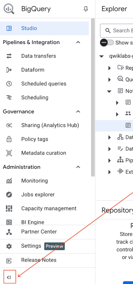
1. 在 Google Cloud 控制台中，前往导航菜单 > BigQuery。

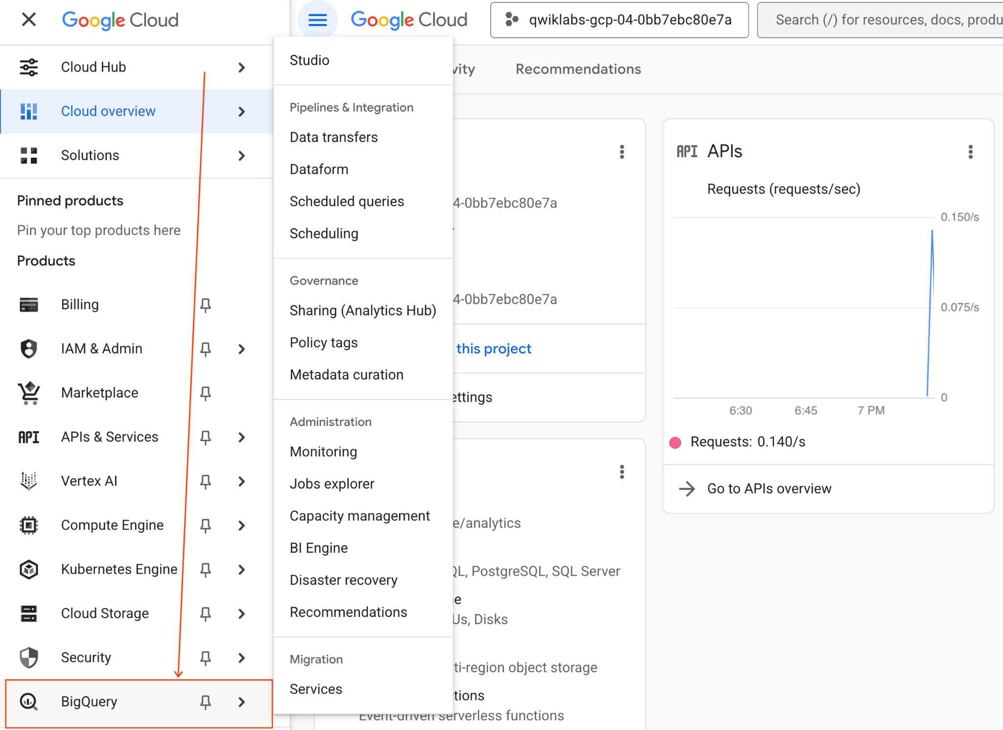
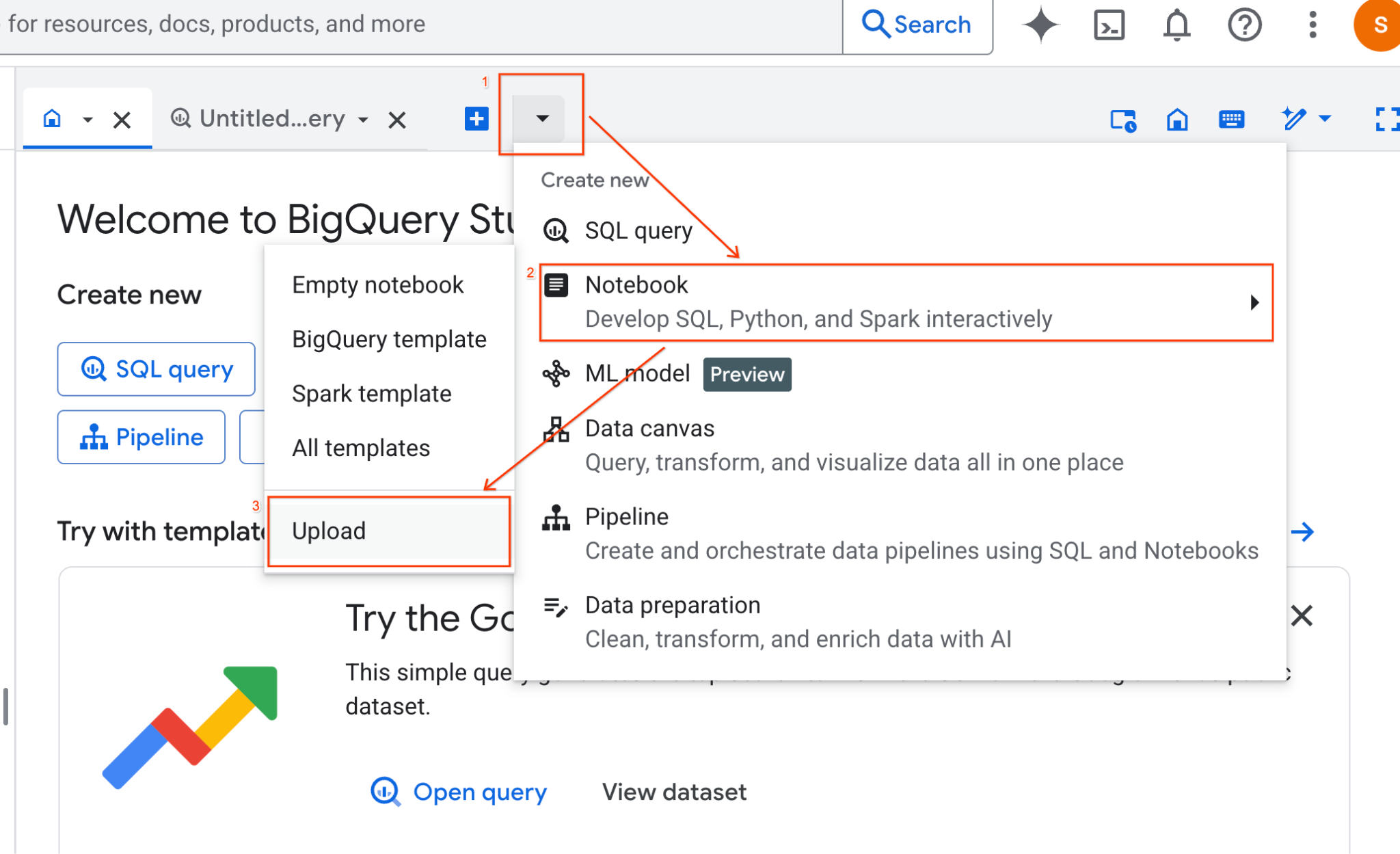
2. 在 BigQuery Studio 窗格中，点击下拉箭头按钮，将鼠标悬停在“笔记本”上，然后选择“上传”。

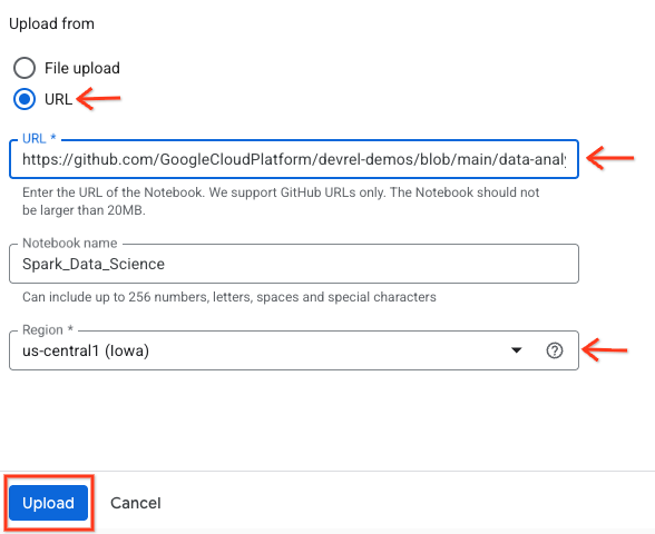
3. 选择“网址”单选按钮，然后输入以下网址：

https://github.com/GoogleCloudPlatform/devrel-demos/blob/main/data-analytics/dataproc-webinar/data-science/Spark_Data_Science.ipynb

4. 将区域设置为 us-central11，然后点击上传 。

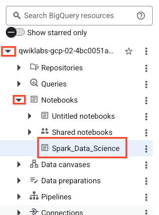
5. 如需打开笔记本，请在探索器 窗格中点击项目 ID 名称旁边的下拉箭头。然后，点击笔记本 的下拉菜单。点击笔记本 Spark_Data_Science。

6. 收起 BigQuery 导航菜单 和笔记本的目录 ，以获得更多空间。

3. 连接到运行时并运行其他设置代码

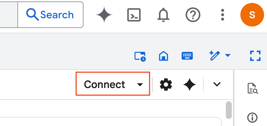
1. 点击连接 。在弹出式窗口中，使用您的电子邮件账号授权 Colab Enterprise。您的笔记本将自动连接到运行时。

注意 ：此过程可能需要几分钟才能完成。

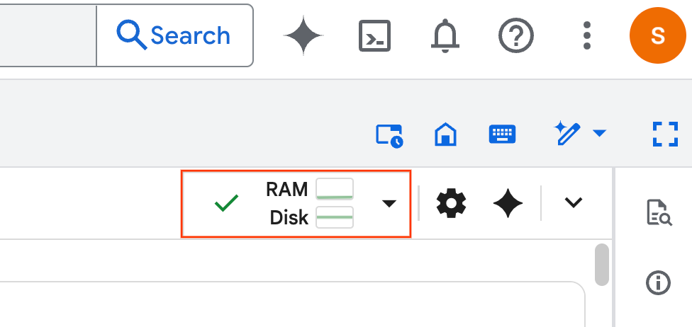
2. 运行时建立后，您将看到以下内容：

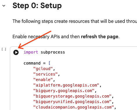
3. 在笔记本中，滚动到设置 部分。从此处开始。

注意 ：打开笔记本并准备就绪后，您现在将主要在 Colab 环境中工作。此笔记本包含整个工作流的所有代码和详细的单元格说明。本实验是一个高级指南，提供简要摘要来帮助您跟踪进度。您可以选择在此处停止阅读 Codelab。

4. 运行设置代码

使用必要的 Python 库配置环境以完成实验。 配置专用 Google 访问通道。创建存储分区。创建 BigQuery 数据集。将项目 ID 复制到笔记本中。选择一个 区域。在本实验中，请使用 us-central1 区域。

您可以通过将光标悬停在代码单元块内并点击箭头来执行代码单元。

# Enable APIs
import subprocess

command = [
    "gcloud",
    "services",
    "enable",
    "aiplatform.googleapis.com",
    "bigquery.googleapis.com",
    "bigquerystorage.googleapis.com",
    "bigqueryunified.googleapis.com",
    "cloudaicompanion.googleapis.com",
    "dataproc.googleapis.com",
    "run.googleapis.com",
    "storage.googleapis.com"
]

result = subprocess.run(command, capture_output=True, text=True)
print(result.stdout)
print(result.stderr)

# Configure a PROJECT_ID and REGION
PROJECT_ID = "<YOUR_PROJECT_ID>"
REGION = "<YOUR_REGION>"

# Enable Private Google Access
import subprocess

command = [
    "gcloud",
    "compute",
    "networks",
    "subnets",
    "update",
    "default",
    f"--region={REGION}",
    "--enable-private-ip-google-access"
]

result = subprocess.run(command, capture_output=True, text=True)
print(result.stdout)
print(result.stderr)

# Create a Cloud Storage Bucket
from google.cloud import storage
from google.cloud.exceptions import NotFound

BUCKET_NAME = f"{PROJECT_ID}-demo"

storage_client = storage.Client(project=PROJECT_ID)
try:
    bucket = storage_client.get_bucket(BUCKET_NAME)
    print(f"Bucket {BUCKET_NAME} already exists.")
except NotFound:
    bucket = storage_client.create_bucket(BUCKET_NAME, location=REGION)
    print(f"Bucket {BUCKET_NAME} created.")


# Create a BigQuery dataset.
from google.cloud import bigquery

DATASET_ID = f"{PROJECT_ID}.demo"

client = bigquery.Client()

dataset = bigquery.Dataset(DATASET_ID)

dataset.location = REGION

dataset = client.create_dataset(dataset, exists_ok=True)

5. 创建与 Google Cloud Serverless for Apache Spark 的连接

使用 Spark Connect，您可以连接到无服务器 Spark 会话以运行交互式 Spark 作业。您可以使用 Lightning Engine 配置运行时，以获得高级 Spark 性能。Lightning Engine 通过使用 Apache Gluten 和 Velox 加速工作负载来工作。

from google.cloud.dataproc_spark_connect import DataprocSparkSession
from google.cloud.dataproc_v1 import Session

session = Session()

session.runtime_config.version = "3.0"

# You can optionally configure Spark properties as well. See https://cloud.google.com/dataproc-serverless/docs/concepts/properties.
session.runtime_config.properties = {
  "dataproc.runtime": "premium",
  "spark.dataproc.engine": "lightningEngine",
}

# To avoid going over quota in this demo, cap the max number of Spark workers.
session.runtime_config.properties = {
    "spark.dynamicAllocation.maxExecutors": "4"
}

spark = (
    DataprocSparkSession.builder
      .appName("CustomSparkSession")
      .dataprocSessionConfig(session)
      .getOrCreate()
)

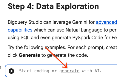
6. 使用 Gemini 加载和探索数据

在本部分中，您将完成任何数据科学项目的第一个重要步骤：准备数据。首先，您将数据从 BigQuery 加载到 Apache Spark 数据帧中。

# Load the tables
order_items = spark.read.format("bigquery").option("table", "bigquery-public-data.thelook_ecommerce.order_items").load()

users = spark.read.format("bigquery").option("table", "bigquery-public-data.thelook_ecommerce.users").load()

# Register temp tables
users.createOrReplaceTempView("users")
order_items.createOrReplaceTempView("order_items")

# Verify temp tables
spark.sql("SELECT * FROM order_items LIMIT 10").show()

然后，您使用 Gemini 生成 PySpark 代码来探索数据并更好地了解数据。

提示 1：使用 PySpark 探索用户表并显示前 10 行。

# prompt:  Using PySpark, explore the users table and show the first 10 rows.

users.show(10)

提示 2：使用 PySpark 探索 order_items 表并显示前 10 行。

# prompt: Using PySpark, explore the order_items table and show the first 10 rows.

order_items.show(10)

提示 3：使用 PySpark 显示用户表中排名前 5 的最常见国家/地区。显示国家/地区以及每个国家/地区的用户数量。

# prompt: Using PySpark, show the top 5 most frequent countries in the users table. Display the country and the number of users from each country.

from pyspark.sql.functions import col, count

users.groupBy("country").agg(count("*").alias("user_count")).orderBy(col("user_count").desc()).limit(5).show()

提示 4：使用 PySpark 查找 order_items 表中商品的平均促销价。

# prompt: Using PySpark, find the average sale price of items in the order_items table.

from pyspark.sql import functions as F

average_sale_price = order_items.agg(F.avg("sale_price").alias("average_sale_price"))
average_sale_price.show()

提示 5：使用“users”表，生成代码以使用合适的绘图库绘制国家/地区与流量来源的关系图。

# prompt: Using the table "users", generate code to plot country vs traffic source using a suitable plotting library.

sql = """
    SELECT
        country,
        traffic_source
    FROM
        `bigquery-public-data.thelook_ecommerce.users`
    WHERE country IS NOT NULL AND traffic_source IS NOT NULL
"""
project_id = "iceberg-summit-2025"
df = pandas_gbq.read_gbq(sql, project_id=project_id, dialect="standard")

import matplotlib.pyplot as plt
import seaborn as sns

# Group by country and traffic_source and count occurrences
df_grouped = df.groupby(['country', 'traffic_source']).size().reset_index(name='count')

# Create a pivot table for easier plotting
pivot_table = df_grouped.pivot(index='country', columns='traffic_source', values='count').fillna(0)

# Plotting
plt.figure(figsize=(15, 8))
pivot_table.plot(kind='bar', stacked=True, figsize=(15, 8))
plt.title('Traffic Source Distribution by Country')
plt.xlabel('Country')
plt.ylabel('Number of Users')
plt.xticks(rotation=90)
plt.legend(title='Traffic Source')
plt.tight_layout()
plt.show()

提示 6 ：创建一个直方图，显示“age”“country”“gender”“traffic_source”的分布情况。

# prompt: Create a histogram showing the distribution of "age", "country", "gender", "traffic_source".

import matplotlib.pyplot as plt

# Convert Spark DataFrame to Pandas DataFrame for visualization
users_pd = users.toPandas()

# Create histograms for 'age', 'country', 'gender', 'traffic_source'
fig, axes = plt.subplots(2, 2, figsize=(15, 10))
fig.suptitle('Distribution of User Attributes')

# Age distribution
axes[0, 0].hist(users_pd['age'].dropna(), bins=20, edgecolor='black')
axes[0, 0].set_title('Age Distribution')
axes[0, 0].set_xlabel('Age')
axes[0, 0].set_ylabel('Number of Users')

# Country distribution
users_pd['country'].value_counts().head(10).plot(kind='bar', ax=axes[0, 1])
axes[0, 1].set_title('Top 10 Countries Distribution')
axes[0, 1].set_xlabel('Country')
axes[0, 1].set_ylabel('Number of Users')
axes[0, 1].tick_params(axis='x', rotation=45)

# Gender distribution
users_pd['gender'].value_counts().plot(kind='bar', ax=axes[1, 0])
axes[1, 0].set_title('Gender Distribution')
axes[1, 0].set_xlabel('Gender')
axes[1, 0].set_ylabel('Number of Users')
axes[1, 0].tick_params(axis='x', rotation=0)

# Traffic Source distribution
users_pd['traffic_source'].value_counts().head(10).plot(kind='bar', ax=axes[1, 1])
axes[1, 1].set_title('Top 10 Traffic Source Distribution')
axes[1, 1].set_xlabel('Traffic Source')
axes[1, 1].set_ylabel('Number of Users')
axes[1, 1].tick_params(axis='x', rotation=45)

plt.tight_layout(rect=[0, 0.03, 1, 0.95])
plt.show()

7. 数据准备和特征工程

接下来，您将对数据执行特征工程。选择适当的列，将数据转换为更合适的数据类型，并确定标签列。

features = spark.sql("""
SELECT
  CAST(u.age AS DOUBLE) AS age,
  CAST(hash(u.country) AS BIGINT) * 1.0 AS country_hash,
  CAST(hash(u.gender) AS BIGINT) * 1.0 AS gender_hash,
  CAST(hash(u.traffic_source) AS BIGINT) * 1.0 AS traffic_source_hash,
  CASE WHEN COUNT(oi.id) > 0 THEN 1 ELSE 0 END AS label -- Changed label generation to count order items
FROM users AS u
LEFT JOIN order_items AS oi
ON u.id = oi.user_id
GROUP BY u.id, u.age, u.country, u.gender, u.traffic_source
""")
features.show()

8. 训练逻辑回归模型

使用 MLlib 训练逻辑回归模型。首先，您使用 VectorAssembler 将数据转换为向量格式。然后，StandardScaler 会缩放特征列以获得更好的性能。然后，您将创建一个对 LogisticRegression 模型的引用并定义超参数。您将这些步骤合并到 Pipeline 对象中，使用 fit() 函数训练模型，并使用 transform() 函数转换数据。

from pyspark.ml.classification import LogisticRegression, LogisticRegressionModel
from pyspark.ml.evaluation import BinaryClassificationEvaluator
from pyspark.ml.feature import VectorAssembler, StandardScaler
from pyspark.ml.pipeline import Pipeline
from pyspark.ml.functions import array_to_vector

#Split Train and Test Data (80:20)
train_data, test_data = features.randomSplit([0.8, 0.2], seed=42)

# Initialize VectorAssembler
assembler = VectorAssembler(
    inputCols=["age", "country_hash", "gender_hash", "traffic_source_hash"],
    outputCol="assembled_features"
)

# Initialize StandardScaler
scaler = StandardScaler(inputCol="assembled_features", outputCol="scaled_features")

# Initialize Logistic Regression model
lr = LogisticRegression(
    maxIter=100,
    regParam=0.2,
    threshold=0.8,
    featuresCol="scaled_features",
    labelCol="label"
)

# Define pipeline
pipeline = Pipeline(stages=[assembler, scaler, lr])

# Fit the model
pipeline_model = pipeline.fit(train_data)

# Transform the dataset using the trained model
transformed_dataset = pipeline_model.transform(test_data)
transformed_dataset.show()

9. 模型评估

评估新转换的数据集。生成 曲线下面积 (AUC) 评估指标。

# Model evaluation
eva = BinaryClassificationEvaluator(metricName="areaUnderPR")
aucPR = eva.evaluate(transformed_dataset)
print(f"AUC PR: {aucPR}")

然后，使用 Gemini 生成 PySpark 代码以可视化模型输出。

提示 1 ：生成代码以绘制精确率-召回率 (PR) 曲线。根据模型的预测计算精确率和召回率，并使用合适的绘图库显示 PR 曲线。

# prompt: Generate code to plot the Precision-Recall (PR) curve. Calculate precision and recall from the model's predictions and display the PR curve using a suitable plotting library.

import matplotlib.pyplot as plt
from sklearn.metrics import precision_recall_curve, auc

# Extract predictions and labels
predictions = transformed_dataset.select("prediction", "label").toPandas()

# Calculate precision and recall
precision, recall, _ = precision_recall_curve(predictions["label"], predictions["prediction"])

# Calculate AUC-PR
pr_auc = auc(recall, precision)

# Plot the PR curve
plt.figure(figsize=(8, 6))
plt.plot(recall, precision, color='blue', lw=2, label=f'PR curve (AUC = {pr_auc:.2f})')
plt.xlabel('Recall')
plt.ylabel('Precision')
plt.title('Precision-Recall Curve')
plt.legend(loc='lower left')
plt.grid(True)
plt.show()

提示 2 ：生成代码以创建混淆矩阵可视化。根据模型的预测计算混淆矩阵，并将其显示为热图或表格，其中包含真正例 (TP)、真负例 (TN)、假正例 (FP) 和假负例 (FN) 的计数。

# prompt: Generate code to create a confusion matrix visualization. Calculate the confusion matrix from the model's predictions and display it as a heat map or a table with counts of true positives (TP), true negatives (TN), false positives (FP), and false negatives (FN).

import pandas as pd
import seaborn as sns
import matplotlib.pyplot as plt
from sklearn.metrics import confusion_matrix

# Extract predictions and labels
predictions_and_labels = transformed_dataset.select("prediction", "label").toPandas()

# Calculate the confusion matrix
cm = confusion_matrix(predictions_and_labels["label"], predictions_and_labels["prediction"])

# Create a DataFrame for better visualization
cm_df = pd.DataFrame(cm,
                     index=['Actual Negative', 'Actual Positive'],
                     columns=['Predicted Negative', 'Predicted Positive'])

# Display the confusion matrix as a table
print("Confusion Matrix:")
print(cm_df)

# Display the confusion matrix as a heatmap
plt.figure(figsize=(8, 6))
sns.heatmap(cm_df, annot=True, fmt='d', cmap='Blues', cbar=False, linewidths=.5)
plt.title('Confusion Matrix')
plt.ylabel('Actual Label')
plt.xlabel('Predicted Label')
plt.show()

# Calculate and display TP, TN, FP, FN
TN, FP, FN, TP = cm.ravel()
print(f"
True Positives (TP): {TP}")
print(f"True Negatives (TN): {TN}")
print(f"False Positives (FP): {FP}")
print(f"False Negatives (FN): {FN}")

10. 将预测写入 BigQuery

使用 Gemini 生成代码，将预测写入 BigQuery 数据集中的新表。

提示 ：使用 Spark 将转换后的数据集写入 BigQuery。

# prompt: Using Spark, write the transformed dataset to BigQuery.

transformed_dataset.write.format("bigquery").option("table", f"{PROJECT_ID}.demo.predictions").mode("overwrite").save()

11. 将模型保存到 Cloud Storage

使用 MLlib 的原生功能将模型保存到 Cloud Storage。推理服务器会从此处加载模型。

MODEL_PATH = "models/prediction_model"
pipeline_model.write().overwrite().save(f"gs://{BUCKET_NAME}/{MODEL_PATH}")

12. 创建推理服务器

Cloud Run 是一种灵活的工具，可用于运行无服务器 Web 应用。它使用 Docker 容器为用户提供最大的自定义能力。在本实验中，一个 Dockerfile 配置为运行由 PySpark 提供支持的 Flask 应用。此容器在 Cloud Run 上运行，以对输入数据执行推理。您可以在此处找到其代码。

克隆包含推理服务器代码的仓库。

!git clone https://github.com/GoogleCloudPlatform/devrel-demos.git

查看 Dockerfile。

FROM python:3.12-slim

# Install OpenJDK-21 (Required for Spark)
RUN apt-get update && \
    apt-get install -y openjdk-21-jre-headless procps && \
    rm -rf /var/lib/apt/lists/*

ENV JAVA_HOME=/usr/lib/jvm/java-21-openjdk-amd64
ENV PORT=8080

WORKDIR /app

COPY requirements.txt .
RUN pip install --no-cache-dir -r requirements.txt

COPY main.py .

CMD ["gunicorn", "--bind", "0.0.0.0:8080", "--workers", "1", "--threads", "8", "--timeout", "0", "main:app"]

查看服务器的 Python 代码。

import os
import json
import logging

from flask import Flask, request, jsonify
from google.cloud import storage
from pyspark.ml import PipelineModel
from pyspark.sql import SparkSession
from pyspark.sql.functions import hash, col

# Configure basic logging
logging.basicConfig(level=logging.INFO, format='%(asctime)s - %(levelname)s - %(message)s')

# --- Initialization: Spark and Model Loading ---
GCS_BUCKET = os.environ.get("GCS_BUCKET")
GCS_MODEL_PATH = os.environ.get("GCS_MODEL_PATH")
LOCAL_MODEL_PATH = "/tmp/model"

try:
    spark = SparkSession.builder \
        .appName("CloudRunSparkService") \
        .master("local[*]") \
        .getOrCreate()
    logging.info("Spark Session successfully initialized.")
except Exception as e:
    logging.error(f"Failed to initialize Spark Session: {e}")
    raise

def download_directory(bucket_name, prefix, local_path):
    """Downloads a directory from GCS to local filesystem."""
    storage_client = storage.Client()
    bucket = storage_client.get_bucket(bucket_name)
    blobs = list(bucket.list_blobs(prefix=prefix))
    
    if len(blobs) == 0:
        logging.error(f"No files found in GCS bucket {bucket_name} at prefix {prefix}")
        return
    
    for blob in blobs:
        if blob.name.endswith("/"): continue # Skip directories
        
        # Structure local paths
        relative_path = os.path.relpath(blob.name, prefix)
        local_file_path = os.path.join(local_path, relative_path)
        os.makedirs(os.path.dirname(local_file_path), exist_ok=True)
        
        blob.download_to_filename(local_file_path)
    print(f"Model downloaded to {local_path}")

# Load model
def load_model(LOCAL_MODEL_PATH, GCS_BUCKET, GCS_MODEL_PATH):
    """Download and load model on startup to avoid latency per request."""
    global MODEL
    if not os.path.exists(LOCAL_MODEL_PATH):
        download_directory(GCS_BUCKET, GCS_MODEL_PATH, LOCAL_MODEL_PATH)
    
    logging.info(f"Loading PySpark model from {GCS_MODEL_PATH}")
    # Load the Spark ML model
    try:
        MODEL = PipelineModel.load(LOCAL_MODEL_PATH)
        logging.info("Spark model loaded successfully.")
    except Exception as e:
        logging.error(f"Failed to load model: {e}")
        raise
    
# Load Model on Startup
load_model(LOCAL_MODEL_PATH, GCS_BUCKET, GCS_MODEL_PATH)

# --- Flask Application Setup ---
app = Flask(__name__)

@app.route('/predict', methods=['POST'])
def predict():
    """
    Handles incoming POST requests for inference.
    Expects JSON data that can be converted into a Spark DataFrame.
    """
    if MODEL is None:
        return jsonify({"error": "Model failed to load at startup."}), 500

    try:
        # 1. Get data from the request
        data = request.get_json()
        
        # 2. Check length of list
        data_len = len(data)
        cap = 100
        if data_len > cap:
            return jsonify({"error": f"Too many records. Count: {data_len}, Max: {cap}"}), 400

        # 2. Create Spark DataFrame
        df = spark.createDataFrame(data)
        
        # 3. Transform data
        input_df = df.select(
            col("age").cast("DOUBLE").alias("age"), 
            (hash(col("country")).cast("BIGINT") * 1.0).alias("country_hash"),
            (hash(col("gender")).cast("BIGINT") * 1.0).alias("gender_hash"),
            (hash(col("traffic_source")).cast("BIGINT") * 1.0).alias("traffic_source_hash")
        )

        # 3. Perform Inference
        predictions_df = MODEL.transform(input_df)

        # 4. Prepare results (collect and serialize)
        results = [p.prediction for p in predictions_df.select("prediction").collect()]

        # 5. Return JSON response
        return jsonify({"predictions": results})

    except Exception as e:
        logging.error(f"An error occurred during prediction: {e}")
        #return jsonify({"error": str(e)}), 500
        raise e  
    
# Gunicorn entry point uses 'app' from this file
if __name__ == '__main__':
    # Local testing only: Cloud Run uses Gunicorn/CMD command
    app.run(host='0.0.0.0', port=int(os.environ.get('PORT', 8080)))

部署推理服务器。

import subprocess

command = [
    "gcloud",
    "run",
    "deploy",
    "inference-server",
    "--source",
    "/content/devrel-demos/data-analytics/dataproc-webinar/data-science/inference-server",
    "--region",
    f"{REGION}",
    "--port",
    "8080",
    "--memory",
    "2Gi",
    "--allow-unauthenticated",
    "--set-env-vars",
    f"GCS_BUCKET={BUCKET_NAME},GCS_MODEL_PATH={MODEL_PATH}",
    "--startup-probe",
    "tcpSocket.port=8080,initialDelaySeconds=240,failureThreshold=3,timeoutSeconds=240,periodSeconds=240"
]

result = subprocess.run(command, capture_output=True, text=True)
print(result.stdout)
print(result.stderr)

将输出中的推理服务器网址复制到新变量中。它类似于 https://inference-server-123456789.us-central1.run.app.

INFERENCE_SERVER_URL = "<YOUR_SERVER_URL>"

测试推理服务器。

import requests

age = "25.0"
country = "United States"
traffic_source = "Search"
gender = "F"

response = requests.post(
    f"{INFERENCE_SERVER_URL}/predict",
    json=[{"age": age, "country": country, "traffic_source": traffic_source, "gender": gender}],
    headers={"Content-Type": "application/json"}
)

print(response.json())

输出应为 1.0 或 0.0。

{'predictions': [1.0]}

13. 配置智能体

使用 Agent Engine 创建可以执行推理的智能体。Agent Engine 是 Vertex AI Platform 的一部分，是一组可让开发者在生产环境中部署、管理和扩缩 AI 智能体的服务。它具有许多工具，包括评估智能体、会话上下文和代码执行。它支持许多热门的智能体框架，包括 智能体开发套件 (ADK)。ADK 是一个开源智能体框架，虽然是为与 Gemini 和 Google 生态系统搭配使用而构建和优化的，但它与模型无关。它的设计旨在让智能体开发更接近于软件开发。

初始化 Vertex AI 客户端。

import vertexai
from vertexai import agent_engines # For the prebuilt templates

client = vertexai.Client(  # For service interactions via client.agent_engines
    project=f"{PROJECT_ID}",
    location=f"{REGION}",
)

定义用于查询已部署模型的函数。

def predict_purchase(
    age: str = "25.0",
    country: str = "United States",
    traffic_source: str = "Search",
    gender: str = "M",
):
    """Predicts whether or not a user will purchase a product.

    Args:
        age: The age of the user.
        country: The country of the user. One of: "China", "Poland", "Germany", "United States", "Spain", "United Kingdom", "España", "Japan", "Brasil", "Colombia", "Belgium", "South Korea", "Austria", "France", "Australia".
        Traffic_source: The source of the user's traffic. One of: "Display", "Email", "Search", "Organic", "Facebook".
        gender: The gender of the user. One of: "M" or "F".

    Returns:
        True if the model output is 1.0, False otherwise.
    """
    import requests
    response = requests.post(
        f"{INFERENCE_SERVER_URL}/predict",
        json=[{"age": age, "country": country, "traffic_source": traffic_source, "gender": gender}],
        headers={"Content-Type": "application/json"}
    )
    return response.json()

通过传入示例参数来测试该函数。

predict_purchase(age=25.0, country="United States", traffic_source="Search", gender="M")

使用 ADK，在下方定义一个智能体，并提供 predict_purchase 函数作为工具。

from google.adk.agents import Agent
from vertexai import agent_engines

agent = Agent(
   model="gemini-2.5-flash",
   name='purchase_prediction_agent',
   tools=[predict_purchase]
)

通过传入查询在本地测试智能体。

app = agent_engines.AdkApp(agent=agent)
async for event in app.async_stream_query(
    user_id="123",
    message="Will a 25 yo male from the United States who came from Search make a purchase? Strictly output 'yes' or 'no'.",
):
    try:
        print(event['content']['parts'][0]['text'])
    except:
      continue

将模型部署到 Agent Engine。

remote_agent = client.agent_engines.create(
    agent=app,
    config={
        "requirements": ["google-cloud-aiplatform[agent_engines,adk]"],
        "staging_bucket": f"gs://{BUCKET_NAME}",
        "display_name": "purchase-predictor",
        "description": "Agent that predicts whether or not a user will purchase a product.",
    }
)

完成后，在 Cloud 控制台 中查看已部署的模型。

再次查询模型。现在，它指向已部署的智能体，而不是本地版本。

async for event in remote_agent.async_stream_query(
    user_id="123",
    message="Will a 25 yo male from the United States who came from Search make a purchase? Strictly output 'yes' or 'no'.",
):
    try:
        print(event['content']['parts'][0]['text'])
    except:
      continue

14. 清理

删除您创建的所有 Google Cloud 资源。运行此类清理命令是一项至关重要的最佳实践，可避免日后产生费用。

# Delete the deployed agent.
remote_agent.delete(force=True)

# Delete the inference server.
import subprocess

command = [
    "gcloud",
    "run",
    "services",
    "delete",
    "inference-server",
    "--region",
    f"{REGION}",
    "--quiet"
]

subprocess.run(command, capture_output=True, text=True)

# Delete the BigQuery dataset.
bigquery_client = bigquery.Client()

bigquery_client.delete_dataset(
    f"{PROJECT_ID}.demo", delete_contents=True, not_found_ok=True
)

# Delete the Storage bucket.
storage_client = storage.Client()

bucket = storage_client.get_bucket(BUCKET_NAME)
bucket.delete_blobs(list(bucket.list_blobs()))
bucket.delete()

15. 恭喜！

您已完成所有步骤！在此 Codelab 中，您执行了以下操作：

• 使用 BigQuery Studio 笔记本运行数据科学工作流。
• 使用 Google Cloud Serverless for Apache Spark 并由 Spark Connect 提供支持，创建与 Apache Spark 的连接。
• 使用 Lightning Engine 将 Apache Spark 工作负载的速度提升高达 4.3 倍。
• 使用 Apache Spark 和 BigQuery 之间的内置集成从 BigQuery 加载数据。
• 使用 Gemini 辅助代码生成功能探索数据。
• 使用 Apache Spark 的数据处理框架执行特征工程。
• 使用 Apache Spark 的原生机器学习库 MLlib 训练和评估分类模型。
• 使用 Flask 和 Cloud Run 为分类模型部署推理服务器
• 使用 Agent Engine 和 智能体开发套件 (ADK) 部署智能体，以使用自然语言查询推理服务器

后续操作

• 详细了解 Google Cloud Serverless for Apache Spark。
• 了解如何配置 Cloud Run。
• 详细了解 Agent Engine。