運用 Spark 執行資料科學作業

1. 總覽

TheLook 是一家假設的電子商務服飾零售商，在 BigQuery 中儲存客戶、產品、訂單、物流、網路事件和數位行銷活動的資料。該公司希望運用團隊現有的 SQL 和 PySpark 專業知識，使用 Apache Spark 分析這項資料。

為避免手動佈建基礎架構或微調 Spark，TheLook 尋求自動調整資源配置解決方案，讓他們專注於工作負載，不必費心管理叢集。此外，他們希望盡量減少整合 Spark 和 BigQuery 的工作量，同時留在 BigQuery Studio 環境中。

在本實驗室中，您將使用 PySpark 建構邏輯迴歸分類器，並運用 BigQuery Studio 的原生筆記本整合功能和 AI 功能探索資料，預測使用者是否會購物。將這個模型部署至推論伺服器，並建立代理程式，以自然語言查詢模型。

必要條件

開始這個實驗室之前，您應已熟悉下列概念：

基本 SQL 和 Python 程式設計。
在 Jupyter 筆記本中執行 Python 程式碼。
對分散式運算有基本瞭解

目標

使用 BigQuery Studio 筆記本執行資料科學工作流程。
使用 Google Cloud Serverless for Apache Spark 建立 Apache Spark 連線，並由 Spark Connect 提供支援。
使用 Lightning Engine 將 Apache Spark 工作負載的速度提升最多 4.3 倍。
使用 Apache Spark 和 BigQuery 之間的內建整合功能，從 BigQuery 載入資料。
使用 Gemini 輔助程式碼生成功能探索資料。
使用 Apache Spark 的資料處理架構執行特徵工程。
使用 Apache Spark 的原生機器學習程式庫 MLlib 訓練及評估分類模型。
使用 Flask 和 Cloud Run 部署分類模型的推論伺服器
使用 Agent Engine 和 Agent Development Kit (ADK) 部署代理，以自然語言查詢推論伺服器，

2. 連線至 Colab 執行階段環境

找出 Google Cloud 專案

建立 Google Cloud 專案。您可以使用現有專案。

啟用建議的 API：

按一下這裡，啟用下列 API：

瀏覽使用者介面：

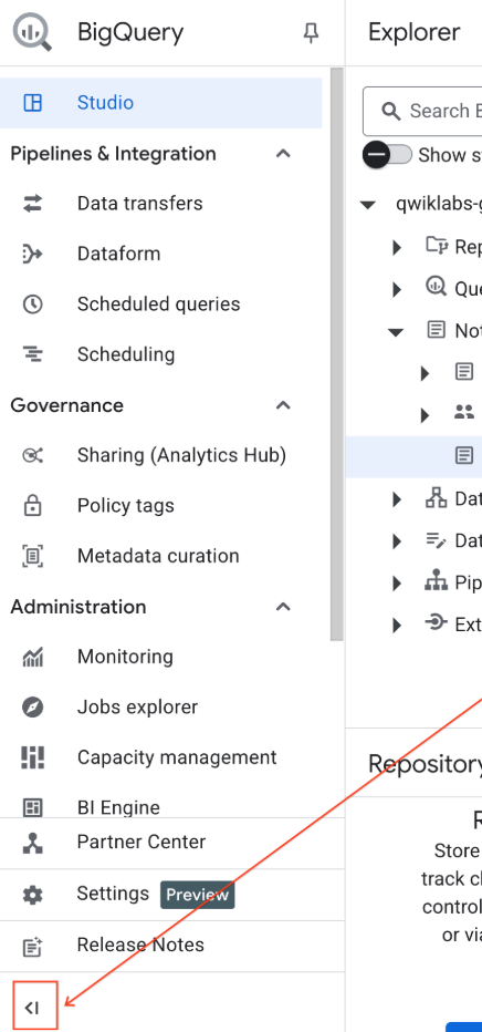
在 Google Cloud 控制台中，依序前往「導覽選單」>「BigQuery」。

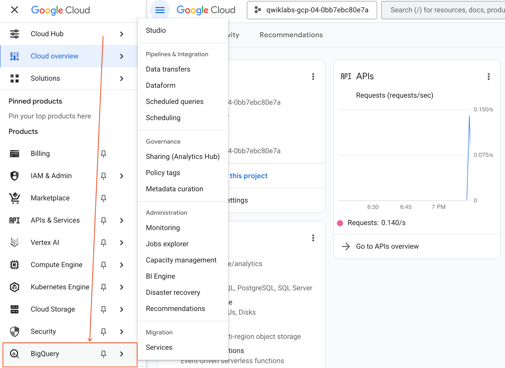
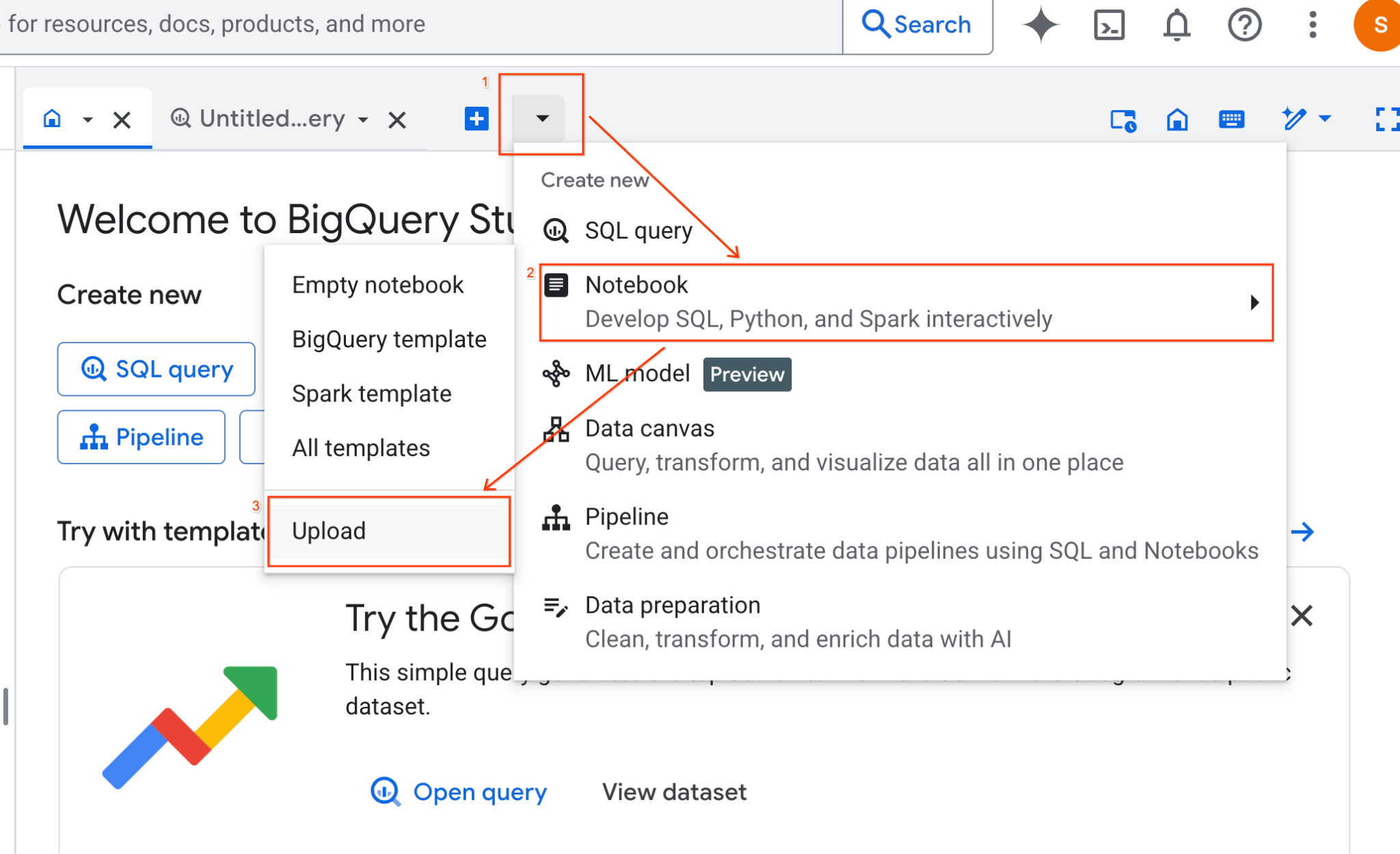
箭頭指向 Google Cloud 控制台中的 BigQuery 分頁。

在 BigQuery Studio 窗格中，按一下下拉式箭頭按鈕，將游標懸停在「筆記本」上，然後選取「上傳」。

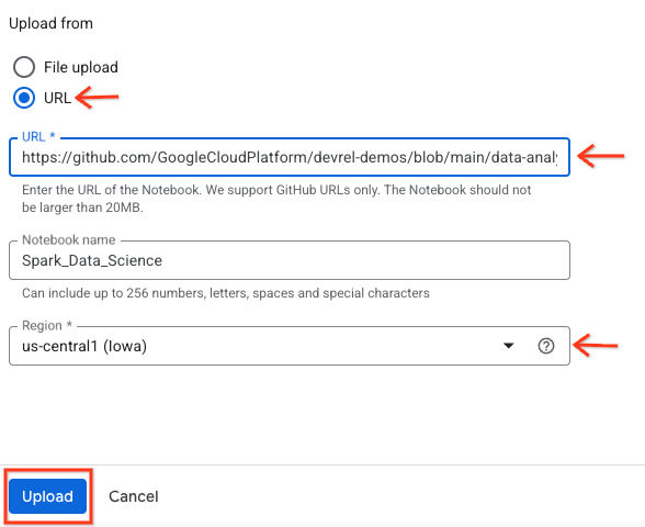
選取「網址」圓形按鈕，然後輸入下列網址：

https://github.com/GoogleCloudPlatform/devrel-demos/blob/main/data-analytics/dataproc-webinar/data-science/Spark_Data_Science.ipynb

將區域設為 us-central11，然後按一下「上傳」。

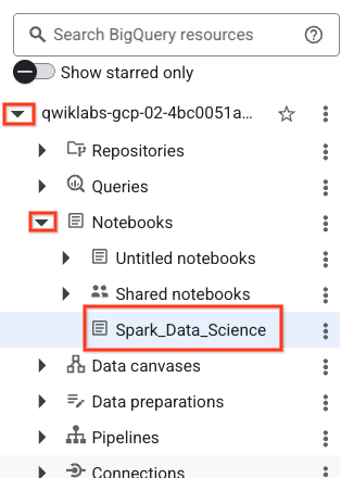
如要開啟筆記本，請在「Explorer」窗格中，點選專案 ID 名稱旁的下拉式箭頭。然後點選「筆記本」的下拉式選單。按一下筆記本 Spark_Data_Science。

收合 BigQuery 導覽選單和筆記本的目錄，爭取更多空間。

3. 連線至執行階段並執行其他設定碼

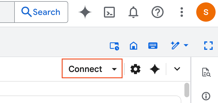
按一下「連結」，在彈出式視窗中，使用電子郵件帳戶授權 Colab Enterprise。筆記本會自動連線至執行階段。

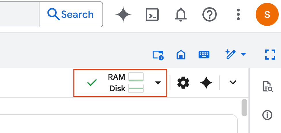
建立執行階段後，您會看到下列內容：

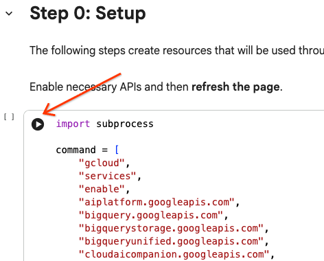
在筆記本中，捲動至「設定」部分。從這裡開始。

4. 執行設定碼

設定環境，安裝完成實驗室所需的 Python 程式庫。設定 Private Google Access。建立 Storage bucket。建立 BigQuery 資料集。將專案 ID 複製到筆記本。選取區域。在本實驗室中，請使用 us-central1 區域。

將游標懸停在儲存格區塊內，然後點選箭頭，即可執行程式碼儲存格。

# Enable APIs
import subprocess

command = [
    "gcloud",
    "services",
    "enable",
    "aiplatform.googleapis.com",
    "bigquery.googleapis.com",
    "bigquerystorage.googleapis.com",
    "bigqueryunified.googleapis.com",
    "cloudaicompanion.googleapis.com",
    "dataproc.googleapis.com",
    "run.googleapis.com",
    "storage.googleapis.com"
]

result = subprocess.run(command, capture_output=True, text=True)
print(result.stdout)
print(result.stderr)

# Configure a PROJECT_ID and REGION
PROJECT_ID = "<YOUR_PROJECT_ID>"
REGION = "<YOUR_REGION>"

# Enable Private Google Access
import subprocess

command = [
    "gcloud",
    "compute",
    "networks",
    "subnets",
    "update",
    "default",
    f"--region={REGION}",
    "--enable-private-ip-google-access"
]

result = subprocess.run(command, capture_output=True, text=True)
print(result.stdout)
print(result.stderr)

# Create a Cloud Storage Bucket
from google.cloud import storage
from google.cloud.exceptions import NotFound

BUCKET_NAME = f"{PROJECT_ID}-demo"

storage_client = storage.Client(project=PROJECT_ID)
try:
    bucket = storage_client.get_bucket(BUCKET_NAME)
    print(f"Bucket {BUCKET_NAME} already exists.")
except NotFound:
    bucket = storage_client.create_bucket(BUCKET_NAME, location=REGION)
    print(f"Bucket {BUCKET_NAME} created.")


# Create a BigQuery dataset.
from google.cloud import bigquery

DATASET_ID = f"{PROJECT_ID}.demo"

client = bigquery.Client()

dataset = bigquery.Dataset(DATASET_ID)

dataset.location = REGION

dataset = client.create_dataset(dataset, exists_ok=True)

5. 建立與 Google Cloud Serverless for Apache Spark 的連線

使用 Spark Connect 連線至無伺服器 Spark 工作階段，即可執行互動式 Spark 工作。您可以透過 Lightning Engine 設定執行階段，進一步提升 Spark 效能。Lightning Engine 會使用 Apache Gluten 和 Velox 加速工作負載。

from google.cloud.dataproc_spark_connect import DataprocSparkSession
from google.cloud.dataproc_v1 import Session

session = Session()

session.runtime_config.version = "3.0"

# You can optionally configure Spark properties as well. See https://cloud.google.com/dataproc-serverless/docs/concepts/properties.
session.runtime_config.properties = {
  "dataproc.runtime": "premium",
  "spark.dataproc.engine": "lightningEngine",
}

# To avoid going over quota in this demo, cap the max number of Spark workers.
session.runtime_config.properties = {
    "spark.dynamicAllocation.maxExecutors": "4"
}

spark = (
    DataprocSparkSession.builder
      .appName("CustomSparkSession")
      .dataprocSessionConfig(session)
      .getOrCreate()
)

6. 使用 Gemini 載入及探索資料

在本節中，您將完成資料科學專案的第一個重要步驟：準備資料。首先，請從 BigQuery 將資料載入 Apache Spark DataFrame。

# Load the tables
order_items = spark.read.format("bigquery").option("table", "bigquery-public-data.thelook_ecommerce.order_items").load()

users = spark.read.format("bigquery").option("table", "bigquery-public-data.thelook_ecommerce.users").load()

# Register temp tables
users.createOrReplaceTempView("users")
order_items.createOrReplaceTempView("order_items")

# Verify temp tables
spark.sql("SELECT * FROM order_items LIMIT 10").show()

接著，您會使用 Gemini 生成 PySpark 程式碼，探索及深入瞭解資料。

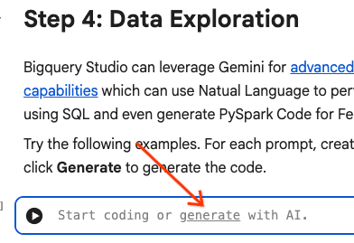
提示 1：使用 PySpark 探索使用者資料表，並顯示前 10 個資料列。

# prompt:  Using PySpark, explore the users table and show the first 10 rows.

users.show(10)

提示 2：使用 PySpark 探索 order_items 資料表，並顯示前 10 列。

# prompt: Using PySpark, explore the order_items table and show the first 10 rows.

order_items.show(10)

提示 3：使用 PySpark，顯示使用者資料表中出現次數最多的前 5 個國家/地區。顯示國家/地區和各國家/地區的使用者人數。

# prompt: Using PySpark, show the top 5 most frequent countries in the users table. Display the country and the number of users from each country.

from pyspark.sql.functions import col, count

users.groupBy("country").agg(count("*").alias("user_count")).orderBy(col("user_count").desc()).limit(5).show()

提示 4：使用 PySpark 找出 order_items 資料表中商品的平均特價。

# prompt: Using PySpark, find the average sale price of items in the order_items table.

from pyspark.sql import functions as F

average_sale_price = order_items.agg(F.avg("sale_price").alias("average_sale_price"))
average_sale_price.show()

提示 5：使用「users」資料表，產生程式碼來繪製國家/地區與流量來源的關係圖，並使用合適的繪圖程式庫。

# prompt: Using the table "users", generate code to plot country vs traffic source using a suitable plotting library.

sql = """
    SELECT
        country,
        traffic_source
    FROM
        `bigquery-public-data.thelook_ecommerce.users`
    WHERE country IS NOT NULL AND traffic_source IS NOT NULL
"""
project_id = "iceberg-summit-2025"
df = pandas_gbq.read_gbq(sql, project_id=project_id, dialect="standard")

import matplotlib.pyplot as plt
import seaborn as sns

# Group by country and traffic_source and count occurrences
df_grouped = df.groupby(['country', 'traffic_source']).size().reset_index(name='count')

# Create a pivot table for easier plotting
pivot_table = df_grouped.pivot(index='country', columns='traffic_source', values='count').fillna(0)

# Plotting
plt.figure(figsize=(15, 8))
pivot_table.plot(kind='bar', stacked=True, figsize=(15, 8))
plt.title('Traffic Source Distribution by Country')
plt.xlabel('Country')
plt.ylabel('Number of Users')
plt.xticks(rotation=90)
plt.legend(title='Traffic Source')
plt.tight_layout()
plt.show()

提示 6：建立直方圖，顯示「年齡」、「國家/地區」、「性別」、「流量來源」的分布情形。

# prompt: Create a histogram showing the distribution of "age", "country", "gender", "traffic_source".

import matplotlib.pyplot as plt

# Convert Spark DataFrame to Pandas DataFrame for visualization
users_pd = users.toPandas()

# Create histograms for 'age', 'country', 'gender', 'traffic_source'
fig, axes = plt.subplots(2, 2, figsize=(15, 10))
fig.suptitle('Distribution of User Attributes')

# Age distribution
axes[0, 0].hist(users_pd['age'].dropna(), bins=20, edgecolor='black')
axes[0, 0].set_title('Age Distribution')
axes[0, 0].set_xlabel('Age')
axes[0, 0].set_ylabel('Number of Users')

# Country distribution
users_pd['country'].value_counts().head(10).plot(kind='bar', ax=axes[0, 1])
axes[0, 1].set_title('Top 10 Countries Distribution')
axes[0, 1].set_xlabel('Country')
axes[0, 1].set_ylabel('Number of Users')
axes[0, 1].tick_params(axis='x', rotation=45)

# Gender distribution
users_pd['gender'].value_counts().plot(kind='bar', ax=axes[1, 0])
axes[1, 0].set_title('Gender Distribution')
axes[1, 0].set_xlabel('Gender')
axes[1, 0].set_ylabel('Number of Users')
axes[1, 0].tick_params(axis='x', rotation=0)

# Traffic Source distribution
users_pd['traffic_source'].value_counts().head(10).plot(kind='bar', ax=axes[1, 1])
axes[1, 1].set_title('Top 10 Traffic Source Distribution')
axes[1, 1].set_xlabel('Traffic Source')
axes[1, 1].set_ylabel('Number of Users')
axes[1, 1].tick_params(axis='x', rotation=45)

plt.tight_layout(rect=[0, 0.03, 1, 0.95])
plt.show()

7. 資料準備和特徵工程

接著，您要對資料執行特徵工程。選取適當的資料欄、將資料轉換為更合適的資料類型，並找出標籤資料欄。

features = spark.sql("""
SELECT
  CAST(u.age AS DOUBLE) AS age,
  CAST(hash(u.country) AS BIGINT) * 1.0 AS country_hash,
  CAST(hash(u.gender) AS BIGINT) * 1.0 AS gender_hash,
  CAST(hash(u.traffic_source) AS BIGINT) * 1.0 AS traffic_source_hash,
  CASE WHEN COUNT(oi.id) > 0 THEN 1 ELSE 0 END AS label -- Changed label generation to count order items
FROM users AS u
LEFT JOIN order_items AS oi
ON u.id = oi.user_id
GROUP BY u.id, u.age, u.country, u.gender, u.traffic_source
""")
features.show()

8. 訓練邏輯迴歸模型

使用 MLlib 訓練邏輯迴歸模型。首先，您會使用 VectorAssembler 將資料轉換為向量格式。接著，StandardScaler 會調整特徵資料欄的比例，以提升效能。接著，您會建立 LogisticRegression 模型的參照，並定義超參數。您會將這些步驟合併為 Pipeline 物件，使用 fit() 函式訓練模型，並使用 transform() 函式轉換資料。

from pyspark.ml.classification import LogisticRegression, LogisticRegressionModel
from pyspark.ml.evaluation import BinaryClassificationEvaluator
from pyspark.ml.feature import VectorAssembler, StandardScaler
from pyspark.ml.pipeline import Pipeline
from pyspark.ml.functions import array_to_vector

#Split Train and Test Data (80:20)
train_data, test_data = features.randomSplit([0.8, 0.2], seed=42)

# Initialize VectorAssembler
assembler = VectorAssembler(
    inputCols=["age", "country_hash", "gender_hash", "traffic_source_hash"],
    outputCol="assembled_features"
)

# Initialize StandardScaler
scaler = StandardScaler(inputCol="assembled_features", outputCol="scaled_features")

# Initialize Logistic Regression model
lr = LogisticRegression(
    maxIter=100,
    regParam=0.2,
    threshold=0.8,
    featuresCol="scaled_features",
    labelCol="label"
)

# Define pipeline
pipeline = Pipeline(stages=[assembler, scaler, lr])

# Fit the model
pipeline_model = pipeline.fit(train_data)

# Transform the dataset using the trained model
transformed_dataset = pipeline_model.transform(test_data)
transformed_dataset.show()

9. 模型評估

評估新轉換的資料集。生成評估指標「曲線下面積 (AUC)」。

# Model evaluation
eva = BinaryClassificationEvaluator(metricName="areaUnderPR")
aucPR = eva.evaluate(transformed_dataset)
print(f"AUC PR: {aucPR}")

接著，使用 Gemini 生成 PySpark 程式碼，將模型輸出內容視覺化。

提示 1：生成程式碼，繪製精確度與喚回度 (PR) 曲線。根據模型的預測結果計算精確度和召回率，並使用合適的繪圖程式庫顯示 PR 曲線。

# prompt: Generate code to plot the Precision-Recall (PR) curve. Calculate precision and recall from the model's predictions and display the PR curve using a suitable plotting library.

import matplotlib.pyplot as plt
from sklearn.metrics import precision_recall_curve, auc

# Extract predictions and labels
predictions = transformed_dataset.select("prediction", "label").toPandas()

# Calculate precision and recall
precision, recall, _ = precision_recall_curve(predictions["label"], predictions["prediction"])

# Calculate AUC-PR
pr_auc = auc(recall, precision)

# Plot the PR curve
plt.figure(figsize=(8, 6))
plt.plot(recall, precision, color='blue', lw=2, label=f'PR curve (AUC = {pr_auc:.2f})')
plt.xlabel('Recall')
plt.ylabel('Precision')
plt.title('Precision-Recall Curve')
plt.legend(loc='lower left')
plt.grid(True)
plt.show()

提示 2：生成程式碼，建立混淆矩陣圖表。根據模型的預測結果計算混淆矩陣，並以熱度圖或表格形式顯示，其中包含真陽性 (TP)、真陰性 (TN)、偽陽性 (FP) 和偽陰性 (FN) 的計數。

# prompt: Generate code to create a confusion matrix visualization. Calculate the confusion matrix from the model's predictions and display it as a heat map or a table with counts of true positives (TP), true negatives (TN), false positives (FP), and false negatives (FN).

import pandas as pd
import seaborn as sns
import matplotlib.pyplot as plt
from sklearn.metrics import confusion_matrix

# Extract predictions and labels
predictions_and_labels = transformed_dataset.select("prediction", "label").toPandas()

# Calculate the confusion matrix
cm = confusion_matrix(predictions_and_labels["label"], predictions_and_labels["prediction"])

# Create a DataFrame for better visualization
cm_df = pd.DataFrame(cm,
                     index=['Actual Negative', 'Actual Positive'],
                     columns=['Predicted Negative', 'Predicted Positive'])

# Display the confusion matrix as a table
print("Confusion Matrix:")
print(cm_df)

# Display the confusion matrix as a heatmap
plt.figure(figsize=(8, 6))
sns.heatmap(cm_df, annot=True, fmt='d', cmap='Blues', cbar=False, linewidths=.5)
plt.title('Confusion Matrix')
plt.ylabel('Actual Label')
plt.xlabel('Predicted Label')
plt.show()

# Calculate and display TP, TN, FP, FN
TN, FP, FN, TP = cm.ravel()
print(f"
True Positives (TP): {TP}")
print(f"True Negatives (TN): {TN}")
print(f"False Positives (FP): {FP}")
print(f"False Negatives (FN): {FN}")

10. 將預測結果寫入 BigQuery

使用 Gemini 生成程式碼，將預測結果寫入 BigQuery 資料集的新資料表。

提示：使用 Spark 將轉換後的資料集寫入 BigQuery。

# prompt: Using Spark, write the transformed dataset to BigQuery.

transformed_dataset.write.format("bigquery").option("table", f"{PROJECT_ID}.demo.predictions").mode("overwrite").save()

11. 將模型儲存至 Cloud Storage

使用 MLlib 的原生功能，將模型儲存至 Cloud Storage。推論伺服器會從這裡載入模型。

MODEL_PATH = "models/prediction_model"
pipeline_model.write().overwrite().save(f"gs://{BUCKET_NAME}/{MODEL_PATH}")

12. 建立推論伺服器

Cloud Run 是一項彈性工具，可執行無伺服器網頁應用程式。並使用 Docker 容器，為使用者提供最大程度的自訂功能。在本實驗室中，Dockerfile 已設定為執行支援 PySpark 的 Flask 應用程式。這個容器會在 Cloud Run 上執行，對輸入資料進行推論。如要查看相關程式碼，請按這裡。

複製存放區，其中包含推論伺服器程式碼。

!git clone https://github.com/GoogleCloudPlatform/devrel-demos.git

查看 Dockerfile。

FROM python:3.12-slim

# Install OpenJDK-21 (Required for Spark)
RUN apt-get update && \
    apt-get install -y openjdk-21-jre-headless procps && \
    rm -rf /var/lib/apt/lists/*

ENV JAVA_HOME=/usr/lib/jvm/java-21-openjdk-amd64
ENV PORT=8080

WORKDIR /app

COPY requirements.txt .
RUN pip install --no-cache-dir -r requirements.txt

COPY main.py .

CMD ["gunicorn", "--bind", "0.0.0.0:8080", "--workers", "1", "--threads", "8", "--timeout", "0", "main:app"]

查看伺服器的 Python 程式碼。

import os
import json
import logging

from flask import Flask, request, jsonify
from google.cloud import storage
from pyspark.ml import PipelineModel
from pyspark.sql import SparkSession
from pyspark.sql.functions import hash, col

# Configure basic logging
logging.basicConfig(level=logging.INFO, format='%(asctime)s - %(levelname)s - %(message)s')

# --- Initialization: Spark and Model Loading ---
GCS_BUCKET = os.environ.get("GCS_BUCKET")
GCS_MODEL_PATH = os.environ.get("GCS_MODEL_PATH")
LOCAL_MODEL_PATH = "/tmp/model"

try:
    spark = SparkSession.builder \
        .appName("CloudRunSparkService") \
        .master("local[*]") \
        .getOrCreate()
    logging.info("Spark Session successfully initialized.")
except Exception as e:
    logging.error(f"Failed to initialize Spark Session: {e}")
    raise

def download_directory(bucket_name, prefix, local_path):
    """Downloads a directory from GCS to local filesystem."""
    storage_client = storage.Client()
    bucket = storage_client.get_bucket(bucket_name)
    blobs = list(bucket.list_blobs(prefix=prefix))
    
    if len(blobs) == 0:
        logging.error(f"No files found in GCS bucket {bucket_name} at prefix {prefix}")
        return
    
    for blob in blobs:
        if blob.name.endswith("/"): continue # Skip directories
        
        # Structure local paths
        relative_path = os.path.relpath(blob.name, prefix)
        local_file_path = os.path.join(local_path, relative_path)
        os.makedirs(os.path.dirname(local_file_path), exist_ok=True)
        
        blob.download_to_filename(local_file_path)
    print(f"Model downloaded to {local_path}")

# Load model
def load_model(LOCAL_MODEL_PATH, GCS_BUCKET, GCS_MODEL_PATH):
    """Download and load model on startup to avoid latency per request."""
    global MODEL
    if not os.path.exists(LOCAL_MODEL_PATH):
        download_directory(GCS_BUCKET, GCS_MODEL_PATH, LOCAL_MODEL_PATH)
    
    logging.info(f"Loading PySpark model from {GCS_MODEL_PATH}")
    # Load the Spark ML model
    try:
        MODEL = PipelineModel.load(LOCAL_MODEL_PATH)
        logging.info("Spark model loaded successfully.")
    except Exception as e:
        logging.error(f"Failed to load model: {e}")
        raise
    
# Load Model on Startup
load_model(LOCAL_MODEL_PATH, GCS_BUCKET, GCS_MODEL_PATH)

# --- Flask Application Setup ---
app = Flask(__name__)

@app.route('/predict', methods=['POST'])
def predict():
    """
    Handles incoming POST requests for inference.
    Expects JSON data that can be converted into a Spark DataFrame.
    """
    if MODEL is None:
        return jsonify({"error": "Model failed to load at startup."}), 500

    try:
        # 1. Get data from the request
        data = request.get_json()
        
        # 2. Check length of list
        data_len = len(data)
        cap = 100
        if data_len > cap:
            return jsonify({"error": f"Too many records. Count: {data_len}, Max: {cap}"}), 400

        # 2. Create Spark DataFrame
        df = spark.createDataFrame(data)
        
        # 3. Transform data
        input_df = df.select(
            col("age").cast("DOUBLE").alias("age"), 
            (hash(col("country")).cast("BIGINT") * 1.0).alias("country_hash"),
            (hash(col("gender")).cast("BIGINT") * 1.0).alias("gender_hash"),
            (hash(col("traffic_source")).cast("BIGINT") * 1.0).alias("traffic_source_hash")
        )

        # 3. Perform Inference
        predictions_df = MODEL.transform(input_df)

        # 4. Prepare results (collect and serialize)
        results = [p.prediction for p in predictions_df.select("prediction").collect()]

        # 5. Return JSON response
        return jsonify({"predictions": results})

    except Exception as e:
        logging.error(f"An error occurred during prediction: {e}")
        #return jsonify({"error": str(e)}), 500
        raise e  
    
# Gunicorn entry point uses 'app' from this file
if __name__ == '__main__':
    # Local testing only: Cloud Run uses Gunicorn/CMD command
    app.run(host='0.0.0.0', port=int(os.environ.get('PORT', 8080)))

部署推論伺服器。

import subprocess

command = [
    "gcloud",
    "run",
    "deploy",
    "inference-server",
    "--source",
    "/content/devrel-demos/data-analytics/dataproc-webinar/data-science/inference-server",
    "--region",
    f"{REGION}",
    "--port",
    "8080",
    "--memory",
    "2Gi",
    "--allow-unauthenticated",
    "--set-env-vars",
    f"GCS_BUCKET={BUCKET_NAME},GCS_MODEL_PATH={MODEL_PATH}",
    "--startup-probe",
    "tcpSocket.port=8080,initialDelaySeconds=240,failureThreshold=3,timeoutSeconds=240,periodSeconds=240"
]

result = subprocess.run(command, capture_output=True, text=True)
print(result.stdout)
print(result.stderr)

從輸出內容將推論伺服器網址複製到新變數中。這與 https://inference-server-123456789.us-central1.run.app.

INFERENCE_SERVER_URL = "<YOUR_SERVER_URL>"

測試推論伺服器。

import requests

age = "25.0"
country = "United States"
traffic_source = "Search"
gender = "F"

response = requests.post(
    f"{INFERENCE_SERVER_URL}/predict",
    json=[{"age": age, "country": country, "traffic_source": traffic_source, "gender": gender}],
    headers={"Content-Type": "application/json"}
)

print(response.json())

輸出內容應為 1.0 或 0.0。

{'predictions': [1.0]}

13. 設定代理程式

使用 Agent Engine 建立可執行推論的代理程式。Agent Engine 是 Vertex AI 平台的一部分，這組服務可讓開發人員在正式環境中部署、管理及調度 AI 代理。其中包含許多工具，包括評估代理程式、工作階段內容和程式碼執行作業。支援許多熱門的代理架構，包括 Agent Development Kit (ADK)。ADK 是開放原始碼的代理框架，雖然專為 Gemini 和 Google 生態系統建構及最佳化，但與模型無關。旨在讓代理開發過程更像軟體開發。

初始化 Vertex AI 用戶端。

import vertexai
from vertexai import agent_engines # For the prebuilt templates

client = vertexai.Client(  # For service interactions via client.agent_engines
    project=f"{PROJECT_ID}",
    location=f"{REGION}",
)

定義查詢已部署模型的函式。

def predict_purchase(
    age: str = "25.0",
    country: str = "United States",
    traffic_source: str = "Search",
    gender: str = "M",
):
    """Predicts whether or not a user will purchase a product.

    Args:
        age: The age of the user.
        country: The country of the user. One of: "China", "Poland", "Germany", "United States", "Spain", "United Kingdom", "España", "Japan", "Brasil", "Colombia", "Belgium", "South Korea", "Austria", "France", "Australia".
        Traffic_source: The source of the user's traffic. One of: "Display", "Email", "Search", "Organic", "Facebook".
        gender: The gender of the user. One of: "M" or "F".

    Returns:
        True if the model output is 1.0, False otherwise.
    """
    import requests
    response = requests.post(
        f"{INFERENCE_SERVER_URL}/predict",
        json=[{"age": age, "country": country, "traffic_source": traffic_source, "gender": gender}],
        headers={"Content-Type": "application/json"}
    )
    return response.json()

傳入範例參數，測試函式。

predict_purchase(age=25.0, country="United States", traffic_source="Search", gender="M")

使用 ADK 在下方定義代理程式，並提供 predict_purchase 函式做為工具。

from google.adk.agents import Agent
from vertexai import agent_engines

agent = Agent(
   model="gemini-2.5-flash",
   name='purchase_prediction_agent',
   tools=[predict_purchase]
)

傳遞查詢內容，在本機測試代理程式。

app = agent_engines.AdkApp(agent=agent)
async for event in app.async_stream_query(
    user_id="123",
    message="Will a 25 yo male from the United States who came from Search make a purchase? Strictly output 'yes' or 'no'.",
):
    try:
        print(event['content']['parts'][0]['text'])
    except:
      continue

將模型部署至 Agent Engine。

remote_agent = client.agent_engines.create(
    agent=app,
    config={
        "requirements": ["google-cloud-aiplatform[agent_engines,adk]"],
        "staging_bucket": f"gs://{BUCKET_NAME}",
        "display_name": "purchase-predictor",
        "description": "Agent that predicts whether or not a user will purchase a product.",
    }
)

完成後，請在 Cloud 控制台中查看已部署的模型。

再次查詢模型。現在會指向已部署的代理程式，而非本機版本。

async for event in remote_agent.async_stream_query(
    user_id="123",
    message="Will a 25 yo male from the United States who came from Search make a purchase? Strictly output 'yes' or 'no'.",
):
    try:
        print(event['content']['parts'][0]['text'])
    except:
      continue

14. 清理

刪除您建立的所有 Google Cloud 資源。執行這類清除指令是重要的最佳做法，可避免日後產生費用。

# Delete the deployed agent.
remote_agent.delete(force=True)

# Delete the inference server.
import subprocess

command = [
    "gcloud",
    "run",
    "services",
    "delete",
    "inference-server",
    "--region",
    f"{REGION}",
    "--quiet"
]

subprocess.run(command, capture_output=True, text=True)

# Delete the BigQuery dataset.
bigquery_client = bigquery.Client()

bigquery_client.delete_dataset(
    f"{PROJECT_ID}.demo", delete_contents=True, not_found_ok=True
)

# Delete the Storage bucket.
storage_client = storage.Client()

bucket = storage_client.get_bucket(BUCKET_NAME)
bucket.delete_blobs(list(bucket.list_blobs()))
bucket.delete()

15. 恭喜！

您成功了！在本程式碼研究室中，您已完成下列事項：

使用 BigQuery Studio 筆記本執行資料科學工作流程。
使用 Google Cloud Serverless for Apache Spark 建立 Apache Spark 連線，並由 Spark Connect 提供支援。
使用 Lightning Engine 將 Apache Spark 工作負載的速度提升 4.3 倍。
使用 Apache Spark 和 BigQuery 之間的內建整合功能，從 BigQuery 載入資料。
使用 Gemini 輔助程式碼生成功能探索資料。
使用 Apache Spark 的資料處理架構執行特徵工程。
使用 Apache Spark 的原生機器學習程式庫 MLlib 訓練及評估分類模型。
使用 Flask 和 Cloud Run 部署分類模型的推論伺服器
使用 Agent Engine 和 Agent Development Kit (ADK) 部署代理，以自然語言查詢推論伺服器，

後續步驟

進一步瞭解 Google Cloud Serverless for Apache Spark。
瞭解如何設定 Cloud Run。
參閱 Agent Engine。