
1. Introduction
In this codelab, you will build a cross-cloud open data lakehouse that unifies data silos across AWS, Google Cloud, and AlloyDB without the need for complex ETL. You will use Lakehouse as the central intelligence hub, AlloyDB as an operational data source, and Managed Service for Apache Spark for high-performance vectorized processing. Finally, you will use Gemini to derive powerful business insights from your lakehouse.
Imagine your transactional data (users, orders, order items) is in an operational AlloyDB database, your product data is in an AWS S3 bucket, and massive clickstream event logs are stored in Cloud Storage. You need to join these datasets to identify target demographics for your next marketing campaign and generate personalized outreach emails.
Prerequisites
- Familiarity with basic SQL and terminal commands.
- A Google Cloud project with billing enabled.
What you'll learn
- How to integrate disparate data silos using BigQuery zero-ETL (AlloyDB) and Lakehouse for Apache Iceberg.
- How to run a high-speed behavioral profiling job using Managed Service for Apache Spark powered by the C++ native Lightning Engine.
- How to use the BigQuery data agent to perform complex natural language analysis on unified data.
- How to configure the Model Context Protocol (MCP) to allow the Gemini CLI to read from your Lakehouse for Apache Iceberg and draft marketing content.
What you'll need
- A Google Cloud Account and Google Cloud Project
- A web browser such as Chrome
What you'll need
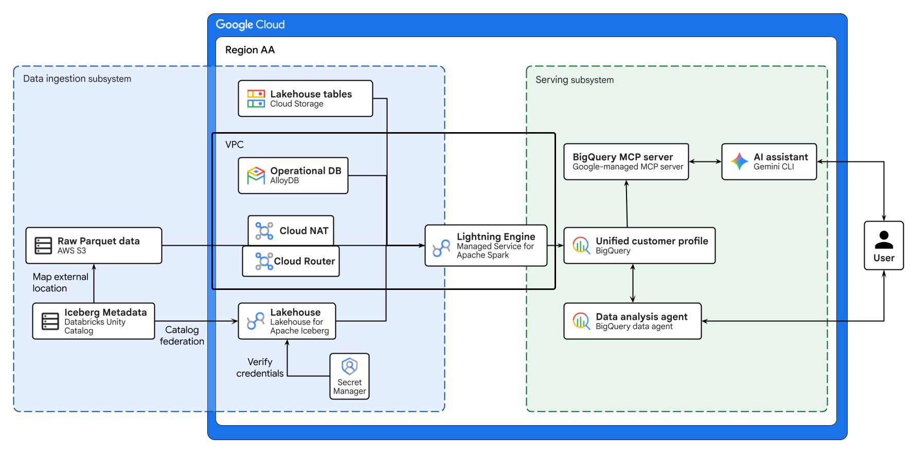
The diagram above illustrates the end-to-end flow of the cross-cloud lakehouse built in this codelab. Operational data from AlloyDB and remote data from AWS S3 are securely federated using Lakehouse for Apache Iceberg. Managed Service for Apache Spark processes these disparate sources to build a unified customer profile in BigQuery. Finally, a BigQuery Data Agent and Google-managed BigQuery MCP server via Gemini CLI provide an intuitive, AI-driven interface for advanced data analysis.
Key concepts
- Cross-cloud open data lakehouse: Unifies data silos across AWS, Google Cloud, and on-premises environments without the need for complex ETL.
- BigQuery zero-ETL: Allows direct querying of operational databases without complex data movement.
- Lakehouse for Apache Iceberg: Enables consistent security and governance across cross-cloud storage using the Apache Iceberg format.
- Lightning Engine: C++ native engine for high-performance Apache Spark execution.
- Model Context Protocol (MCP): Connects Gemini directly to your BigQuery lakehouse.
2. Setup and requirements
Create a Google Cloud Project
- In the Google Cloud Console, on the project selector page, select or create a Google Cloud project.
- Make sure that billing is enabled for your Cloud project. Learn how to check if billing is enabled on a project.
Start Cloud Shell
While Google Cloud can be operated remotely from your laptop, in this codelab you will be using Google Cloud Shell, a command line environment running in the Cloud.
From the Google Cloud Console, click the Cloud Shell icon on the top right toolbar:

It should only take a few moments to provision and connect to the environment. When it is finished, you should see something like this:
This virtual machine is loaded with all the development tools you'll need. It offers a persistent 5GB home directory, and runs on Google Cloud, greatly enhancing network performance and authentication. All of your work in this codelab can be done within a browser. You do not need to install anything.
Initialize environment
Open Cloud Shell and set your project variables to ensure all commands target the correct infrastructure.
cat << 'EOF' > env.sh
#!/bin/bash
# env.sh: Environment variables

export PROJECT_ID=$(gcloud config get-value project)
export REGION="us-west1"
export NETWORK_NAME="default"

export BUCKET_NAME="lakehouse-data-${PROJECT_ID}"
export BQ_DATASET="demo_lakehouse"
export BQ_RESOURCE_CONN="lakehouse-iceberg-conn"
export BQ_ALLOYDB_CONN="alloydb-fed-conn"

export ALLOYDB_CLUSTER="demo-alloy-cluster"
export ALLOYDB_INSTANCE="demo-alloy-primary"
export ALLOYDB_PASSWORD="SuperSecretPassword123!"
export ALLOYDB_DB_NAME="retail_db"

# Multi-cloud configuration identifiers
export SECRET_NAME="dbx-oauth-secret"
export CATALOG_NAME="aws_dbx_catalog"
EOF
Apply the variables to your active session:
source ./env.sh
Enable APIs
Enable the necessary Google Cloud services.
gcloud services enable \
  geminidataanalytics.googleapis.com \
  cloudaicompanion.googleapis.com \
  compute.googleapis.com \
  biglake.googleapis.com \
  bigquery.googleapis.com \
  bigqueryconnection.googleapis.com \
  alloydb.googleapis.com \
  servicenetworking.googleapis.com \
  secretmanager.googleapis.com \
  dataplex.googleapis.com \
  datacatalog.googleapis.com \
  dataform.googleapis.com \
  dataproc.googleapis.com --quiet
3. Set up core infrastructure
Instead of moving all data into a single repository via fragile ETL pipelines, you will build a federated cross-cloud architecture. In a real-world enterprise, data is inherently fragmented due to differing system requirements. You will orchestrate the following data sources:
- AlloyDB (Core transactional DB): Stores users, orders, and order_items data. As a live operational database, it guarantees ACID properties required for financial transactions and profile updates.
- AWS S3 (Master data): Stores
productscatalog. Representing a legacy master data management (MDM) system on AWS. - Google Cloud Storage (Massive data lake): Stores
events(clickstream logs). High-throughput data like web logs would crash a relational database. Object storage provides infinite scalability, and keeping it in Google Cloud maximizes compute locality for your analytical engines.
First, configure the underlying network. Google Cloud managed databases like AlloyDB require a private VPC peering connection to communicate securely within your project network.
# Allocate an IP range for Google Cloud managed services
gcloud compute addresses create google-managed-services-${NETWORK_NAME} \
    --global \
    --purpose=VPC_PEERING \
    --prefix-length=24 \
    --network=projects/${PROJECT_ID}/global/networks/${NETWORK_NAME}

# Establish the VPC peering connection
gcloud services vpc-peerings connect \
    --service=servicenetworking.googleapis.com \
    --ranges=google-managed-services-${NETWORK_NAME} \
    --network=${NETWORK_NAME} \
    --project=${PROJECT_ID}
Next, create a BigQuery dataset and a Lakehouse cloud resource connection. Architecturally, a resource connection delegates data access to a dedicated Google-managed service account, enforcing the principle of least privilege.
# Create the central data lakehouse dataset
bq mk --dataset --location=${REGION} ${PROJECT_ID}:${BQ_DATASET}
gcloud storage buckets create gs://${BUCKET_NAME} --location=${REGION}

# Create a Lakehouse resource connection
bq mk --connection --location=${REGION} \
    --connection_type=CLOUD_RESOURCE ${BQ_RESOURCE_CONN}

# Retrieve the automatically provisioned service account
CONN_SA=$(bq show --connection --format=json ${PROJECT_ID}.${REGION}.${BQ_RESOURCE_CONN} | jq -r '.cloudResource.serviceAccountId')

# Grant the service account permissions to read/write to the data lake
gcloud projects add-iam-policy-binding ${PROJECT_ID} \
    --member="serviceAccount:${CONN_SA}" \
    --role="roles/storage.admin" \
    --quiet
4. Provision the operational database
Provision an AlloyDB primary instance and inject your mission-critical transactional data.
# Create the AlloyDB cluster
gcloud alloydb clusters create ${ALLOYDB_CLUSTER} \
    --region=${REGION} \
    --password=${ALLOYDB_PASSWORD} \
    --network=projects/${PROJECT_ID}/global/networks/${NETWORK_NAME}

# Create the primary instance
gcloud alloydb instances create ${ALLOYDB_INSTANCE} \
    --cluster=${ALLOYDB_CLUSTER} \
    --region=${REGION} \
    --instance-type=PRIMARY \
    --cpu-count=2 \
    --assign-inbound-public-ip=ASSIGN_IPV4 \
    --database-flags=password.enforce_complexity=on
Once the database is ready, you must create a BigQuery external connection to AlloyDB. This connection securely stores the database credentials and endpoint, allowing BigQuery to push down SQL execution directly to the AlloyDB compute engine (zero-ETL).
# Create the BigQuery to AlloyDB connection
bq mk --connection --location=${REGION} --project_id=${PROJECT_ID} \
  --connector_configuration "{
    \"connector_id\": \"google-alloydb\",
    \"asset\": {
      \"database\": \"${ALLOYDB_DB_NAME}\",
      \"google_cloud_resource\": \"//alloydb.googleapis.com/projects/${PROJECT_ID}/locations/${REGION}/clusters/${ALLOYDB_CLUSTER}/instances/${ALLOYDB_INSTANCE}\"
    },
    \"authentication\": {
      \"username_password\": {
        \"username\": \"postgres\",
        \"password\": { \"plaintext\": \"${ALLOYDB_PASSWORD}\" }
      }
    }
  }" ${BQ_ALLOYDB_CONN}

# Grant the BigQuery connection service agent permission to access AlloyDB
PROJECT_NUMBER=$(gcloud projects describe ${PROJECT_ID} --format="value(projectNumber)")
BQ_SERVICE_AGENT="service-${PROJECT_NUMBER}@gcp-sa-bigqueryconnection.iam.gserviceaccount.com"

gcloud projects add-iam-policy-binding ${PROJECT_ID} \
    --member="serviceAccount:${BQ_SERVICE_AGENT}" \
    --role="roles/alloydb.client" \
    --quiet
Securely push the transactional tables into AlloyDB. Use the AlloyDB Auth Proxy to securely connect your local Cloud Shell session to the private AlloyDB instance. This allows you to push the transactional data using local command-line tools.
# Extract full raw data to Cloud Storage using the BigQuery extract API
bq extract --destination_format=CSV --print_header=true "bigquery-public-data:thelook_ecommerce.users" gs://${BUCKET_NAME}/tmp/users.csv
bq extract --destination_format=CSV --print_header=true "bigquery-public-data:thelook_ecommerce.orders" gs://${BUCKET_NAME}/tmp/orders.csv
bq extract --destination_format=CSV --print_header=true "bigquery-public-data:thelook_ecommerce.order_items" gs://${BUCKET_NAME}/tmp/order_items.csv

# Download the CSVs to the local Cloud Shell session
gcloud storage cp gs://${BUCKET_NAME}/tmp/users.csv .
gcloud storage cp gs://${BUCKET_NAME}/tmp/orders.csv .
gcloud storage cp gs://${BUCKET_NAME}/tmp/order_items.csv .

# Download and start the AlloyDB auth proxy
curl -sL "https://storage.googleapis.com/alloydb-auth-proxy/v1.13.11/alloydb-auth-proxy.linux.amd64" -o alloydb-auth-proxy && chmod +x alloydb-auth-proxy

./alloydb-auth-proxy projects/${PROJECT_ID}/locations/${REGION}/clusters/${ALLOYDB_CLUSTER}/instances/${ALLOYDB_INSTANCE} --public-ip &
PROXY_PID=$!
sleep 15 # Wait for the proxy to fully initialize

# Create the database
export PGPASSWORD=${ALLOYDB_PASSWORD}
psql -h 127.0.0.1 -p 5432 -U postgres -c "CREATE DATABASE ${ALLOYDB_DB_NAME};" || true

# Load into AlloyDB mimicking the exact schema via heredoc
psql -h 127.0.0.1 -p 5432 -U postgres -d ${ALLOYDB_DB_NAME} << 'EOF'
CREATE TABLE IF NOT EXISTS users (id INT PRIMARY KEY, first_name VARCHAR(255), last_name VARCHAR(255), email VARCHAR(255), age INT, gender VARCHAR(50), state VARCHAR(100), street_address VARCHAR(255), postal_code VARCHAR(50), city VARCHAR(100), country VARCHAR(100), latitude FLOAT, longitude FLOAT, traffic_source VARCHAR(100), created_at TIMESTAMP, user_geom TEXT);

CREATE TABLE IF NOT EXISTS orders (order_id INT PRIMARY KEY, user_id INT, status VARCHAR(50), gender VARCHAR(50), created_at TIMESTAMP, returned_at TIMESTAMP, shipped_at TIMESTAMP, delivered_at TIMESTAMP, num_of_item INT);

CREATE TABLE IF NOT EXISTS order_items (id INT PRIMARY KEY, order_id INT, user_id INT, product_id INT, inventory_item_id INT, status VARCHAR(50), created_at TIMESTAMP, shipped_at TIMESTAMP, delivered_at TIMESTAMP, returned_at TIMESTAMP, sale_price FLOAT);

\copy users FROM 'users.csv' WITH (FORMAT csv, HEADER true)
\copy orders FROM 'orders.csv' WITH (FORMAT csv, HEADER true)
\copy order_items FROM 'order_items.csv' WITH (FORMAT csv, HEADER true)
EOF

# Clean up local temporary files and Cloud Storage artifacts
kill $PROXY_PID && rm -f users.csv orders.csv order_items.csv alloydb-auth-proxy
gcloud storage rm gs://${BUCKET_NAME}/tmp/*.csv
5. Federate the master data (AWS spoke)
Our product catalog, containing raw item metadata, natively resides on AWS S3 as Apache Iceberg tables. The metadata is governed by a remote catalog.
Instead of building fragile ETL pipelines to copy this data into Google Cloud, you will use Lakehouse for Apache Iceberg (REST catalog federation).
This zero-ETL approach allows Lakehouse and Managed Service for Apache Spark to dynamically discover and read the Iceberg metadata and underlying Parquet files directly from your remote environment.
If you have an active AWS account and Databricks Unity Catalog configured, you may use that. Otherwise, you can mock your environment using Google Cloud Storage. Choose one or the other.
Option A: Bring your own AWS (Native Apache Iceberg)
Prerequisite: This option assumes you have already provisioned an AWS S3 bucket, connected it as an external location in Databricks Unity Catalog, mapped an Iceberg table, and generated an OAuth service principal with read access.
1. Secure credential storage
Hardcoding long-lived access tokens is an architectural anti-pattern. You will store the Databricks OAuth client ID and secret in Google Cloud Secret Manager. The Lakehouse service will fetch these dynamically at runtime to vend short-lived tokens, centralizing your credential governance.
Run the following block to generate the script. (Do not edit anything yet).
cat << 'EOF' > create_secret.sh
#!/bin/bash
source ./env.sh

# Define your Databricks OAuth credentials
DATABRICKS_CLIENT_ID="<YOUR_DATABRICKS_CLIENT_ID>"
DATABRICKS_CLIENT_SECRET="<YOUR_DATABRICKS_CLIENT_SECRET>"
DATABRICKS_WORKSPACE="<YOUR_WORKSPACE>.cloud.databricks.com" # Exclude https://
DATABRICKS_CATALOG="google_lakehouse_catalog"

# Define the secure credentials payload
export CLOUDSDK_API_ENDPOINT_OVERRIDES_SECRETMANAGER="https://secretmanager.${REGION}.rep.googleapis.com/"
SECRET_PAYLOAD="{ \"client_id\": \"${DATABRICKS_CLIENT_ID}\", \"client_secret\": \"${DATABRICKS_CLIENT_SECRET}\" }"

# Pipe the JSON payload into Google Cloud Secret Manager
echo "$SECRET_PAYLOAD" | gcloud secrets create ${SECRET_NAME} \
  --location=${REGION} \
  --project=${PROJECT_ID} \
  --data-file=-
EOF
Then, run the following command to automatically open the generated script in the visual code editor above your terminal.
cloudshell edit create_secret.sh
- In the editor, replace the
<YOUR_...>placeholders with your actual Databricks credentials. - Ensure your workspace URL does not include
https://or trailing slashes (e.g.,123456789.cloud.databricks.com). - Press
Ctrl+S(orCmd+Son Mac) to save the file. - Return to your terminal session and execute the script:
source create_secret.sh
2. Create the federated catalog
For simplicity in this codelab, you will configure the catalog to securely traverse the public internet. However, for production workloads, querying massive datasets over the public internet incurs unnecessary egress costs and unpredictable latency. Best practice mandates configuring a private Cross-Cloud Interconnect (CCI) between AWS and Google Cloud, which significantly reduces egress costs and ensures deterministic network performance.
Use the gcloud CLI to provision the federated Lakehouse catalog:
# Execute the Lakehouse CLI to provision the federated catalog
gcloud alpha biglake iceberg catalogs create ${CATALOG_NAME} \
    --project="${PROJECT_ID}" \
    --primary-location="${REGION}" \
    --catalog-type="federated" \
    --federated-catalog-type="unity" \
    --secret-name="projects/${PROJECT_ID}/locations/${REGION}/secrets/${SECRET_NAME}" \
    --unity-instance-name="${DATABRICKS_WORKSPACE}" \
    --unity-catalog-name="${DATABRICKS_CATALOG}" \
    --refresh-interval="330s"
3. Apply Least Privilege IAM Bindings
When you provisioned the federated catalog in the previous step, Google Cloud Lakehouse automatically launched a background refresh job to synchronize the Iceberg manifests every 330 seconds.
You must grant the secretAccessor role to the Lakehouse catalog service account so it can securely fetch the Databricks OAuth token during these background syncs and query executions. Missing this binding will result in silent 403 errors when Lakehouse attempts to update the catalog.
# Extract the automatically provisioned Lakehouse catalog service account
LAKEHOUSE_SA=$(curl -s -X GET "https://biglake.googleapis.com/iceberg/v1/restcatalog/extensions/projects/${PROJECT_ID}/catalogs/${CATALOG_NAME}" \
  -H "Authorization: Bearer $(gcloud auth application-default print-access-token)" | jq -r '."biglake-service-account"')

# Grant the secretAccessor role for background metadata synchronization and query execution
gcloud secrets add-iam-policy-binding ${SECRET_NAME} \
  --project=${PROJECT_ID} --location=${REGION} \
  --member="serviceAccount:${LAKEHOUSE_SA}" \
  --role="roles/secretmanager.secretAccessor" --quiet
4. Enable Outbound Internet for Managed Service for Apache Spark
In a subsequent step, Managed Service for Apache Spark will read the remote AWS data. Because Managed Service for Apache Spark Serverless runs entirely within a private VPC network without external IP addresses, it cannot reach AWS S3 over the internet by default. You must provision a Cloud NAT to allow the Spark workers outbound internet access.
# Create a Cloud Router
gcloud compute routers create lakehouse-router \
    --network=${NETWORK_NAME} \
    --region=${REGION}

# Create a Cloud NAT attached to the router
gcloud compute routers nats create lakehouse-nat \
    --router=lakehouse-router \
    --auto-allocate-nat-external-ips \
    --nat-all-subnet-ip-ranges \
    --region=${REGION}
5. Define the downstream target
Export this variable so downstream Apache Spark jobs know exactly where to query the AWS data without requiring manual code changes.
# Assuming your schema is 'retail' and table is 'aws_products'
export AWS_PRODUCTS_TABLE="${CATALOG_NAME}.retail.aws_products"

# Persist the variable for future shell sessions
echo "export AWS_PRODUCTS_TABLE=\"${AWS_PRODUCTS_TABLE}\"" >> env.sh
Option B: Mock AWS environment via Cloud Storage
If you do not have an active AWS account, you can simulate the cross-cloud silo natively using Lakehouse managed tables on Google Cloud Storage.
1. Create the mock Iceberg table
# Copy raw products data to a temporary BigQuery table
bq cp --force bigquery-public-data:thelook_ecommerce.products ${PROJECT_ID}:${BQ_DATASET}.temp_products_raw

# Create an open Iceberg table using the Lakehouse cloud resource connection
bq query --use_legacy_sql=false "
CREATE OR REPLACE TABLE \`${PROJECT_ID}.${BQ_DATASET}.aws_products\`
WITH CONNECTION \`${REGION}.${BQ_RESOURCE_CONN}\`
OPTIONS (file_format = 'PARQUET', table_format = 'ICEBERG', storage_uri = 'gs://${BUCKET_NAME}/aws_products')
AS SELECT * FROM \`${PROJECT_ID}.${BQ_DATASET}.temp_products_raw\`;"

# Cleanup temporary table
bq rm -f -t ${PROJECT_ID}:${BQ_DATASET}.temp_products_raw
2. Define the downstream target
Standard BigQuery datasets use a 3-part namespace structure (project.dataset.table). Export this variable so the downstream Apache Spark job targets the mock data.
export AWS_PRODUCTS_TABLE="${PROJECT_ID}.${BQ_DATASET}.aws_products"

# Persist the variable for future shell sessions
echo "export AWS_PRODUCTS_TABLE=\"${AWS_PRODUCTS_TABLE}\"" >> env.sh
6. Ingest event logs (Google Cloud spoke)
Clickstream data grows exponentially. You store the complete, unaggregated raw events locally in Cloud Storage as Managed Lakehouse tables.
bq cp --force bigquery-public-data:thelook_ecommerce.events ${PROJECT_ID}:${BQ_DATASET}.temp_events_raw

bq query --use_legacy_sql=false "
CREATE OR REPLACE TABLE \`${PROJECT_ID}.${BQ_DATASET}.google_events\`
WITH CONNECTION \`${REGION}.${BQ_RESOURCE_CONN}\`
OPTIONS (file_format = 'PARQUET', table_format = 'ICEBERG', storage_uri = 'gs://${BUCKET_NAME}/google_events')
AS SELECT * FROM \`${PROJECT_ID}.${BQ_DATASET}.temp_events_raw\`;"

bq rm -f -t ${PROJECT_ID}:${BQ_DATASET}.temp_events_raw
7. Build a unified customer profile
With your raw infrastructure fully populated, it is time to build a unified customer profile.
You will utilize Managed Service for Apache Spark powered by Lightning Engine. Lightning Engine is Google Cloud's high-performance C++ native query accelerator, built on open-source technologies like Apache Gluten and Velox, that automatically boosts execution by maximizing CPU efficiency and intelligently caching data. This approach is ideal when performing massive multi-way joins, complex windowing, or behavioral aggregations across multiple clouds.
You will use the Spark BigQuery connector to directly read the federated AlloyDB zero-ETL queries and Lakehouse tables, perform the massive vectorized aggregations natively in Spark, and write the resulting unified profile back to BigQuery.
Configure IAM Permissions for Managed Service for Apache Spark
By default, Serverless Spark executes batch jobs using the Compute Engine default service account. Before submitting the job, you must grant this service account the required permissions to execute the workload and manage BigQuery jobs.
(Note: While the service name has changed to Managed Service for Apache Spark to reflect industry-standard terminology, the underlying API commands and IAM roles still use the dataproc identifier).
# Retrieve the project number to construct the Compute Engine default service account
PROJECT_NUMBER=$(gcloud projects describe ${PROJECT_ID} --format="value(projectNumber)")
export COMPUTE_SA="${PROJECT_NUMBER}-compute@developer.gserviceaccount.com"

# Grant the Managed Service for Apache Spark Worker role to allow job execution
gcloud projects add-iam-policy-binding ${PROJECT_ID} \
    --member="serviceAccount:${COMPUTE_SA}" \
    --role="roles/dataproc.worker" \
    --quiet

# Grant the BigQuery Admin role to allow reading, writing, and querying external connections
gcloud projects add-iam-policy-binding ${PROJECT_ID} \
    --member="serviceAccount:${COMPUTE_SA}" \
    --role="roles/bigquery.admin" \
    --quiet
Create and submit the job
First, create the PySpark job script. This script automatically detects whether you chose Option A (AWS Federated Catalog) or Option B (Google Cloud Mock) based on your AWS_PRODUCTS_TABLE environment variable, defines the Spark SQL logic, and utilizes Spark's native array manipulation to calculate the RFM (recency, frequency, monetary) windows.
Run the following block in Cloud Shell.
# Determine which option was selected based on the AWS_PRODUCTS_TABLE variable
if [[ "${AWS_PRODUCTS_TABLE}" == *"${CATALOG_NAME:-undefined}"* ]]; then
  echo "=> Option A (AWS Federated Catalog) detected."
  export IS_AWS_CATALOG="True"
  export OAUTH_TOKEN=$(gcloud auth print-access-token)
else
  echo "=> Option B (Google Cloud Mock) detected."
  export IS_AWS_CATALOG="False"
  export OAUTH_TOKEN=""
fi

# Create the PySpark script with safely injected variables
cat << EOF > spark_lakehouse_join.py
from pyspark.sql import SparkSession

# --- Environment Variables dynamically injected ---
PROJECT_ID = "${PROJECT_ID}"
CATALOG_NAME = "${CATALOG_NAME}"
OAUTH_TOKEN = "${OAUTH_TOKEN}"
BUCKET_NAME = "${BUCKET_NAME}"
BQ_DATASET = "${BQ_DATASET}"
REGION = "${REGION}"
BQ_ALLOYDB_CONN = "${BQ_ALLOYDB_CONN}"
AWS_PRODUCTS_TABLE = "${AWS_PRODUCTS_TABLE}"
IS_AWS_CATALOG = ${IS_AWS_CATALOG}
# ---------------------------------------------------

# 1. Initialize SparkSession (Dynamic Configuration)
packages =[
    "org.apache.iceberg:iceberg-spark-runtime-3.5_2.12:1.4.3",
    "org.apache.iceberg:iceberg-aws-bundle:1.4.3",
    "org.apache.hadoop:hadoop-aws:3.3.4",
    "com.amazonaws:aws-java-sdk-bundle:1.12.262",
    "com.google.cloud.spark:spark-bigquery-with-dependencies_2.12:0.36.1"
]

builder = SparkSession.builder \\
    .config("spark.sql.extensions", "org.apache.iceberg.spark.extensions.IcebergSparkSessionExtensions") \\
    .config("spark.dataproc.lightningEngine.runtime", "native") \\
    .config("spark.hadoop.fs.gs.velox.client.table-cache-max-size", "0") \\
    .config("spark.jars.packages", ",".join(packages))

# Conditionally configure Lakehouse REST Catalog for Option A
if IS_AWS_CATALOG:
    builder = builder \\
        .config(f"spark.sql.catalog.{CATALOG_NAME}", "org.apache.iceberg.spark.SparkCatalog") \\
        .config(f"spark.sql.catalog.{CATALOG_NAME}.type", "rest") \\
        .config(f"spark.sql.catalog.{CATALOG_NAME}.uri", "https://biglake.googleapis.com/iceberg/v1/restcatalog") \\
        .config(f"spark.sql.catalog.{CATALOG_NAME}.warehouse", f"bl://projects/{PROJECT_ID}/catalogs/{CATALOG_NAME}") \\
        .config(f"spark.sql.catalog.{CATALOG_NAME}.io-impl", "org.apache.iceberg.aws.s3.S3FileIO") \\
        .config(f"spark.sql.catalog.{CATALOG_NAME}.header.X-Iceberg-Access-Delegation", "vended-credentials") \\
        .config(f"spark.sql.catalog.{CATALOG_NAME}.header.x-goog-user-project", PROJECT_ID) \\
        .config(f"spark.sql.catalog.{CATALOG_NAME}.header.Authorization", f"Bearer {OAUTH_TOKEN}") \\
        .config(f"spark.sql.catalog.{CATALOG_NAME}.rest-metrics-reporting-enabled", "false")

spark = builder.getOrCreate()

spark.conf.set("temporaryGcsBucket", BUCKET_NAME)
spark.conf.set("viewsEnabled", "true")
spark.conf.set("materializationDataset", BQ_DATASET)

# 2. Extract operational data via AlloyDB Zero-ETL
users_df = spark.read.format("bigquery").option("query", f"""SELECT id AS user_id, age, country FROM EXTERNAL_QUERY("{REGION}.{BQ_ALLOYDB_CONN}", "SELECT id, age, country FROM users")""").load()
orders_df = spark.read.format("bigquery").option("query", f"""SELECT user_id, order_id, CAST(created_at AS TIMESTAMP) AS order_date FROM EXTERNAL_QUERY("{REGION}.{BQ_ALLOYDB_CONN}", "SELECT user_id, order_id, created_at FROM orders WHERE status = 'Complete'")""").load()
items_df = spark.read.format("bigquery").option("query", f"""SELECT order_id, product_id, sale_price FROM EXTERNAL_QUERY("{REGION}.{BQ_ALLOYDB_CONN}", "SELECT order_id, product_id, sale_price FROM order_items")""").load()

# 3. Read AWS Products (Option A vs B) & Google Cloud Logs
if IS_AWS_CATALOG:
    products_df = spark.table(AWS_PRODUCTS_TABLE)
else:
    products_df = spark.read.format("bigquery").option("table", AWS_PRODUCTS_TABLE).load()

events_df = spark.read.format("bigquery").option("table", f"{PROJECT_ID}.{BQ_DATASET}.google_events").load()

# Register Temp Views
users_df.createOrReplaceTempView("live_user_profiles")
orders_df.createOrReplaceTempView("live_transactions")
items_df.createOrReplaceTempView("live_order_items")
products_df.createOrReplaceTempView("raw_aws_products")
events_df.createOrReplaceTempView("google_events")

# 4. Multi-cloud Distributed Join
unified_profile_df = spark.sql("""
WITH aws_master_catalog AS (
  SELECT id AS product_id, category, brand
  FROM raw_aws_products
),
google_behavioral_logs AS (
  SELECT user_id,
         COUNT(DISTINCT session_id) AS total_sessions,
         COUNT(CASE WHEN event_type = 'cart' THEN 1 END) AS cart_adds
  FROM google_events
  WHERE user_id IS NOT NULL
  GROUP BY user_id
),
user_purchases AS (
  SELECT
    t.user_id, t.order_date, t.order_id, oi.sale_price,
    COALESCE(p.category, 'Unknown') AS category,
    COALESCE(p.brand, 'Unknown') AS brand
  FROM live_transactions t
  JOIN live_order_items oi ON t.order_id = oi.order_id
  LEFT JOIN aws_master_catalog p ON oi.product_id = p.product_id
),
rfm_base AS (
  SELECT
    user_id,
    MAX(order_date) AS last_purchase_date,
    COUNT(DISTINCT order_id) AS total_orders,
    SUM(sale_price) AS lifetime_value
  FROM user_purchases
  GROUP BY user_id
),
ranked_items AS (
  SELECT
    user_id, category, brand, sale_price,
    ROW_NUMBER() OVER(PARTITION BY user_id ORDER BY sale_price DESC) as rn
  FROM user_purchases
),
top_items AS (
  SELECT
    user_id,
    COLLECT_LIST(NAMED_STRUCT('category', category, 'brand', brand, 'sale_price', sale_price)) AS top_preferences
  FROM ranked_items
  WHERE rn <= 3
  GROUP BY user_id
)
SELECT
  CURRENT_TIMESTAMP() AS snapshot_date,
  u.user_id, u.age, u.country,
  r.last_purchase_date,
  COALESCE(r.total_orders, 0) AS total_orders,
  COALESCE(ROUND(r.lifetime_value, 2), 0.0) AS lifetime_value,
  COALESCE(b.total_sessions, 0) AS total_sessions,
  COALESCE(b.cart_adds, 0) AS cart_adds,
  t.top_preferences
FROM live_user_profiles u
LEFT JOIN rfm_base r ON u.user_id = r.user_id
LEFT JOIN top_items t ON u.user_id = t.user_id
LEFT JOIN google_behavioral_logs b ON u.user_id = b.user_id
""")

unified_profile_df.show()

# 5. Write back to BigQuery native partitioned table
(unified_profile_df.write
    .format("bigquery")
    .option("table", f"{PROJECT_ID}.{BQ_DATASET}.unified_customer_profile")
    .option("partitionField", "snapshot_date")
    .option("partitionType", "DAY")
    .option("writeMethod", "direct")
    .mode("overwrite")
    .save())
EOF
With the script fully assembled and the required configurations dynamically injected, submit the batch job to Managed Apache Spark Serverless.
gcloud dataproc batches submit pyspark spark_lakehouse_join.py \
    --project=${PROJECT_ID} \
    --region=${REGION} \
    --version=2.3 \
    --subnet=${NETWORK_NAME} \
    --deps-bucket=${BUCKET_NAME} \
    --properties="dataproc.tier=premium,spark.dataproc.lightningEngine.runtime=native"
Verify job execution in the console
Once the batch job is submitted, you can verify that it is utilizing the accelerated C++ execution engine:
- In the Google Cloud console, navigate to Managed Service for Apache Spark > Serverless > Batches.
- Click on the job that is currently running.
- In the job details pane, verify that the Tier property is set to
Premiumand Engine is set toLightning Engine.
8. Analyze with BigQuery data agent
Now that you have federated the fragmented cross-cloud data and executed the heavy behavioral aggregations using Managed Service for Apache Spark, the next step is data analysis.
First, inspect the schema of the newly created unified profile table in the BigQuery UI to visually understand the data structure you are exposing to the agent:
- In the Google Cloud console, navigate to BigQuery.
- In the Explorer pane on the left, expand your project and the
demo_lakehousedataset. - Click on the
unified_customer_profiletable. - Select the Schema tab in the main workspace.
Check the schema of the new table. The top_preferences column is a REPEATED STRUCT (an array of records containing category, brand, and sale_price). Traditionally, querying nested arrays requires complex SQL using the UNNEST() function, which can be a hurdle for business analysts. By grounding a BigQuery data agent in this specific table, the agent inherently understands the schema and handles complex Google Standard SQL operations under the hood.
Create the data agent
In this section, you will create and interact with a BigQuery data agent. Instead of manually writing complex SQL to unnest arrays and calculate metrics, you will provision an AI agent scoped specifically to your newly created unified profile, allowing for natural language data exploration.
- In the left navigation pane, locate and click on Agents.
- Click + New Agent to initialize a new AI assistant.
- Configure the Agent:
- Agent Name:
Retail VIP Analysis Agent - Data Sources: Click Add Source, and search
unified_customer_profiletable.
- Click Add and wait a few seconds for the Agent to initialize its workspace.
Once the agent is established, defining explicit System Instructions is a critical data governance practice. Use the System Instructions as a Semantic Layer. By embedding enterprise-wide business definitions, handling schema complexities, and establishing analytical guardrails, you abstract technical complexity away from the end-user and prevent the LLM from drawing conclusions from statistically insignificant data.
Paste the following into the Instruction field:
You are an expert Data Analyst specializing in e-commerce customer retention.
Your primary data source is the `unified_customer_profile` table.

Strict Schema Rules:
- The `top_preferences` column is a REPEATED STRUCT (ARRAY).
- Whenever you analyze product categories, brands, or prices, you MUST explicitly use the UNNEST() function on `top_preferences` to access the underlying fields.

Semantic Layer & Business Definitions:
- "At-Risk VIP": Define this specific user cohort as anyone meeting ALL of the following criteria: `lifetime_value` > 100, `cart_adds` > 0, and `last_purchase_date` is more than 90 days ago.

Analytical Guardrails:
- Prioritize statistical significance. When generating business insights based on geographic or demographic groupings, explicitly ignore or deprioritize segments with negligible sample sizes (e.g., countries with very few users) to prevent skewed marketing strategies.
Prompt the agent
Because the complex business logic (the exact definition of an "At-Risk VIP") and the schema handling requirements are securely governed by the System Instructions, the data analyst does not need to write a verbose, condition-heavy prompt.
In the chat interface, enter the following prompt:
Find the total count of At-Risk VIPs grouped by country. For each country, extract the single most frequent product category based on their top preferences. Order the results by the user count in descending order.
Evaluate the generated insight
After submitting the prompt, carefully review the natively generated output to evaluate how the BigQuery Data Agent enforced your System Instructions, acting as both a governed semantic layer and an analytical guardrail.
First, read the summary text generated above the data. Notice how the agent automatically translates your simple request for "At-Risk VIPs" into the exact metric thresholds defined in your System Instructions (e.g., referencing lifetime_value > 100, cart_adds > 0, and 90 days of inactivity). This confirms the agent internalized your business logic, meaning end-users never need to memorize or hardcode complex logic in their daily prompts.
Next, expand the SQL view to inspect the generated code. The agent should have constructed mathematically sound Google Standard SQL based on your instructions:
- Dynamic Time Windows: Look for the timestamp calculation in the
WHEREclause (typically usingTIMESTAMP_SUB(CURRENT_TIMESTAMP(), INTERVAL 90 DAY)). - Strict Schema Adherence: Confirm that the agent obeyed your strict schema rules by explicitly applying the
UNNEST()function to thetop_preferencesarray. To accurately isolate the single most frequent category per country, you will typically see it utilize advanced techniques like aROW_NUMBER() OVER()window function within a Common Table Expression (CTE).
Review the automatically rendered chart and data table. The data will visually reveal your core retention markets (typically highlighting high-volume countries like China or the United States) alongside their universally dominant product affinities (frequently "Jeans"). Notice how the native UI structures the output for immediate consumption without requiring explicit visualization code.
Read through the bulleted Insights text generated by the agent. Because you established Analytical Guardrails, look specifically for an insight regarding Data Quality or Statistical Significance. You might see the agent explicitly flagging countries at the bottom of the table with very low user counts (e.g., regions with only a handful of users). Instead of blindly hallucinating a targeted marketing campaign based on a single data point, the agent will correctly advise that these anomalies are statistically insignificant for a large-scale strategy. This demonstrates how embedding governance guardrails directly into the agent effectively prevents AI-driven business miscalculations.
9. Generate AI insights with Gemini and MCP
The agent has successfully identified the primary target demographic: at-risk VIPs in specific countries. However, an analyst's job stops at the insight. To re-engage these users, the marketing team must execute a campaign.
You will use the Model Context Protocol (MCP) to connect an external AI assistant directly to this specific demographic list in BigQuery, transitioning from data analysis to AI-driven action without building custom APIs.
Configure the BigQuery MCP server
Run the block below to generate the mcp.json configuration file. This file supplies the necessary connection parameters so that the Gemini CLI can safely interface with BigQuery.
mkdir -p ~/.gemini

cat << EOF > ~/.gemini/settings.json
{
  "mcpServers": {
    "bigquery": {
      "httpUrl": "https://bigquery.googleapis.com/mcp",
      "authProviderType": "google_credentials",
      "oauth": {
        "scopes": [
          "https://www.googleapis.com/auth/bigquery"
        ]
      }
    }
  }
}
EOF
Generate a Marketing Email
Start the Gemini CLI tool from your terminal, explicitly passing the MCP configuration flag to allow it to read your BigQuery lakehouse.
Run the Gemini CLI.
source env.sh
gemini
Once the prompt opens, ask it to draft a personalized outreach for your target demographic:
Analyze the demo_lakehouse.unified_customer_profile table in BigQuery. Find exactly one 'country and age group' target demographic that has a high average order value (sale_price >= $80) but a relatively low total revenue compared to others. Then, draft a highly engaging, premium VIP promotional email tailored to this specific demographic. Use $PROJECT_ID to get the current project id.
Gemini will automatically query BigQuery via the MCP server, identify the demographic, and draft the email for you!
10. Cleaning up your environment
To avoid ongoing charges to your Google Cloud account and cleanly reset your project for future runs, you must delete the resources created during this codelab.
Run the following block to create the cleanup.sh script. This script acts as an automated teardown mechanism, permanently removing the AlloyDB cluster and instance, BigQuery datasets, and your Cloud Storage bucket to prevent further billing.
cat << 'EOF' > cleanup.sh
#!/bin/bash
source ./env.sh

echo "=> Deleting BigQuery Dataset (${BQ_DATASET})..."
bq rm -r -f -d ${PROJECT_ID}:${BQ_DATASET} || true

echo "=> Deleting Lakehouse resource connection (${BQ_RESOURCE_CONN})..."
bq rm --connection --project_id=${PROJECT_ID} --location=${REGION} ${BQ_RESOURCE_CONN} || true

echo "=> Deleting AlloyDB connection (${BQ_ALLOYDB_CONN})..."
bq rm --connection --project_id=${PROJECT_ID} --location=${REGION} ${BQ_ALLOYDB_CONN} || true

echo "=> Deleting AlloyDB Instance (${ALLOYDB_INSTANCE}) - This takes a few minutes..."
gcloud alloydb instances delete ${ALLOYDB_INSTANCE} --cluster=${ALLOYDB_CLUSTER} --region=${REGION} --quiet || true

echo "=> Deleting AlloyDB Cluster (${ALLOYDB_CLUSTER})..."
gcloud alloydb clusters delete ${ALLOYDB_CLUSTER} --region=${REGION} --force --quiet || true

echo "=> Deleting Cloud Storage bucket (${BUCKET_NAME})..."
gcloud storage rm -r gs://${BUCKET_NAME} || true

echo "=> Deleting Lakehouse Federated Catalog (if created in Option A)..."
curl -s -X DELETE "https://biglake.googleapis.com/iceberg/v1/restcatalog/extensions/projects/${PROJECT_ID}/catalogs/aws_dbx_catalog" \
   -H "Authorization: Bearer $(gcloud auth application-default print-access-token)" || true

echo "=> Deleting Secret Manager Regional Secret (if created in Option A)..."
CLOUDSDK_API_ENDPOINT_OVERRIDES_SECRETMANAGER="https://secretmanager.${REGION}.rep.googleapis.com/" \
gcloud secrets delete dbx-oauth-secret --location=${REGION} --project=${PROJECT_ID} --quiet || true

echo "=> Deleting Cloud NAT and Router (if created in Option A)..."
gcloud compute routers nats delete lakehouse-nat --router=lakehouse-router --region=${REGION} --quiet || true
gcloud compute routers delete lakehouse-router --region=${REGION} --quiet || true

echo "=> Deleting Service Networking VPC Peering..."
gcloud compute networks peerings delete servicenetworking-googleapis-com \
    --network=${NETWORK_NAME} \
    --project=${PROJECT_ID} --quiet || true

echo "=> Deleting Allocated IP Range for Managed Services..."
gcloud compute addresses delete google-managed-services-${NETWORK_NAME} \
    --global \
    --project=${PROJECT_ID} --quiet || true

echo "=> Removing local temporary files..."
rm -f spark_lakehouse_join.py users.csv orders.csv order_items.csv alloydb-auth-proxy env.sh cleanup.sh ~/.gemini/settings.json

echo "============================================="
echo " TEARDOWN COMPLETED."
echo "============================================="
EOF
Run the cleanup script to safely delete your resources:
bash cleanup.sh
11. Congratulations!
You have successfully built and queried a cross-cloud open data lakehouse.
You learned:
- How to federate data from disparate sources using BigQuery Zero-ETL and Google Cloud Lakehouse.
- How to leverage the C++ native Lightning Engine in Managed Service for Apache Spark's massive vectorized joins.
- How to use the BigQuery Data Agent for natural language exploration.
- How to bridge your data to Gemini using the Model Context Protocol (MCP) and Gemini.
What's Next?
- Explore Lakehouse documentation
- Learn more about AlloyDB zero-ETL to BigQuery
- Read about the Lightning Engine