Real-time Retail Recommendations with Spanner AI and Graph

1. Introduction

This codelab will guide you through using Spanner's AI and graph capabilities to enhance an existing retail database. You'll learn practical techniques for utilizing machine learning within Spanner to better serve your customers. Specifically, we'll implement k-Nearest Neighbors (kNN) and Approximate Nearest Neighbors (ANN) to discover new products that align with individual customer needs. You will also integrate an LLM to provide clear, natural-language explanations for why a specific product recommendation was made.

Beyond recommendation, we'll dive into Spanner's graph functionality. You'll use graph queries to model relationships between products based on customer purchase history and product descriptions. This approach allows for discovering deeply related items, significantly improving the relevance and effectiveness of your "Customers also bought" or "Related items" features. By the end of this codelab, you will have the skills to build an intelligent, scalable, and responsive retail application powered entirely by Google Cloud Spanner.

Scenario

You work for an electronics equipment retailer. Your e-commerce site has a standard Spanner database with Products, Orders, and OrderItems.

A customer lands on your site with a specific need: "I'd like to buy a high performance keyboard. I sometimes code while I'm at the beach so it may get wet."

Your goal is to use Spanner's advanced features to answer this request intelligently:

1. Find: Go beyond simple keyword search to find products whose descriptions semantically match the user's request using vector search.
2. Explain: Use an LLM to analyze the top matches and explain why the recommendation is a good fit, building customer trust.
3. Relate: Use graph queries to find other products that customers frequently purchased along with that recommendation.

2. Before you begin

1. Create a Project In the Google Cloud Console, on the project selector page, select or create a Google Cloud project.
2. Enable Billing Make sure that billing is enabled for your Cloud project. Learn how to check if billing is enabled on a project.
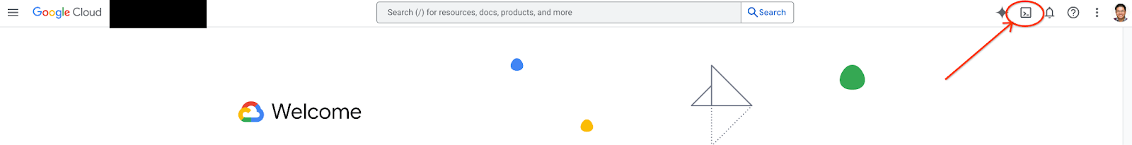
3. Activate Cloud Shell Activate Cloud Shell by clicking the "Activate Cloud Shell" button in the console. You can toggle between the Cloud Shell Terminal and Editor.

4. Authorize and Set Project Once connected to Cloud Shell, check that you're authenticated and that the project is set to your project ID.

gcloud auth list
gcloud config list project

5. If your project is not set, use the following command to set it, replacing <PROJECT_ID> with your actual project ID:

export PROJECT_ID=<PROJECT_ID>
gcloud config set project $PROJECT_ID

6. Enable Required APIs Enable the Spanner, Vertex AI, and Compute Engine APIs. This might take a few minutes.

gcloud services enable \
    spanner.googleapis.com \
    aiplatform.googleapis.com \
    compute.googleapis.com

7. Set a few environment variables that you will reuse.

export INSTANCE_ID=my-first-spanner
export INSTANCE_CONFIG=regional-us-central1

8. Create a free trial Spanner instance if you don't already have a Spanner instance . You'll need a Spanner instance to host your database. We will be using regional-us-central1 as the configuration. You can update this if you would like.

gcloud spanner instances create $INSTANCE_ID \
   --instance-type=free-instance --config=$INSTANCE_CONFIG \
   --description="Trial Instance" 

3. Architectural Overview

Spanner encapsulates all of the necessary functionality except the models which are hosted on Vertex AI.

4. Step 1: Set up the Database and submit your first query.

First, we need to create our database, load our sample retail data, and tell Spanner how to communicate with Vertex AI.

For this section, you'll use the SQL scripts below.

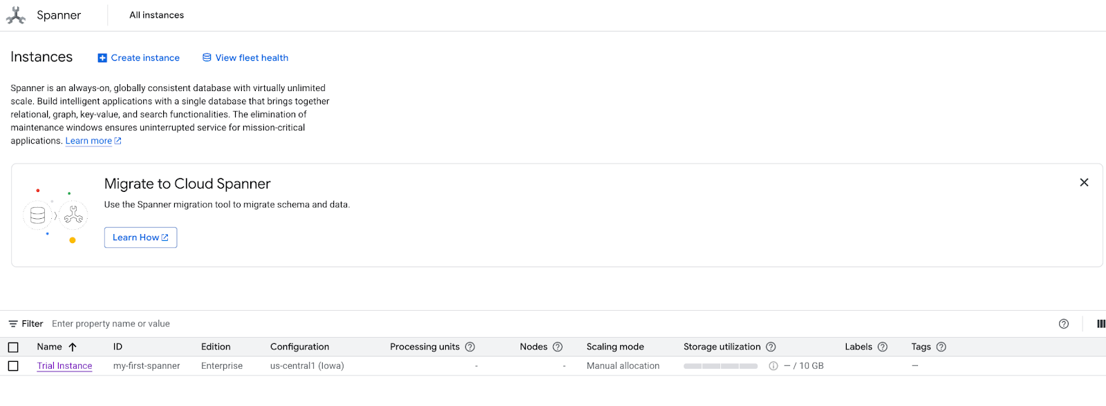
1. Navigate to Spanner's product page.
2. Select the correct instance.

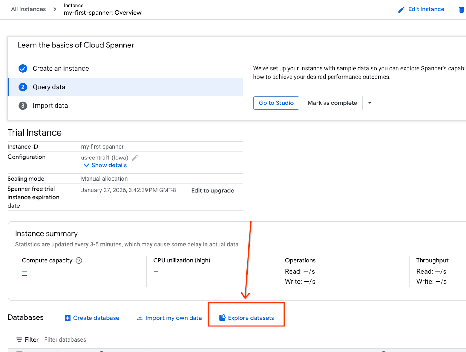
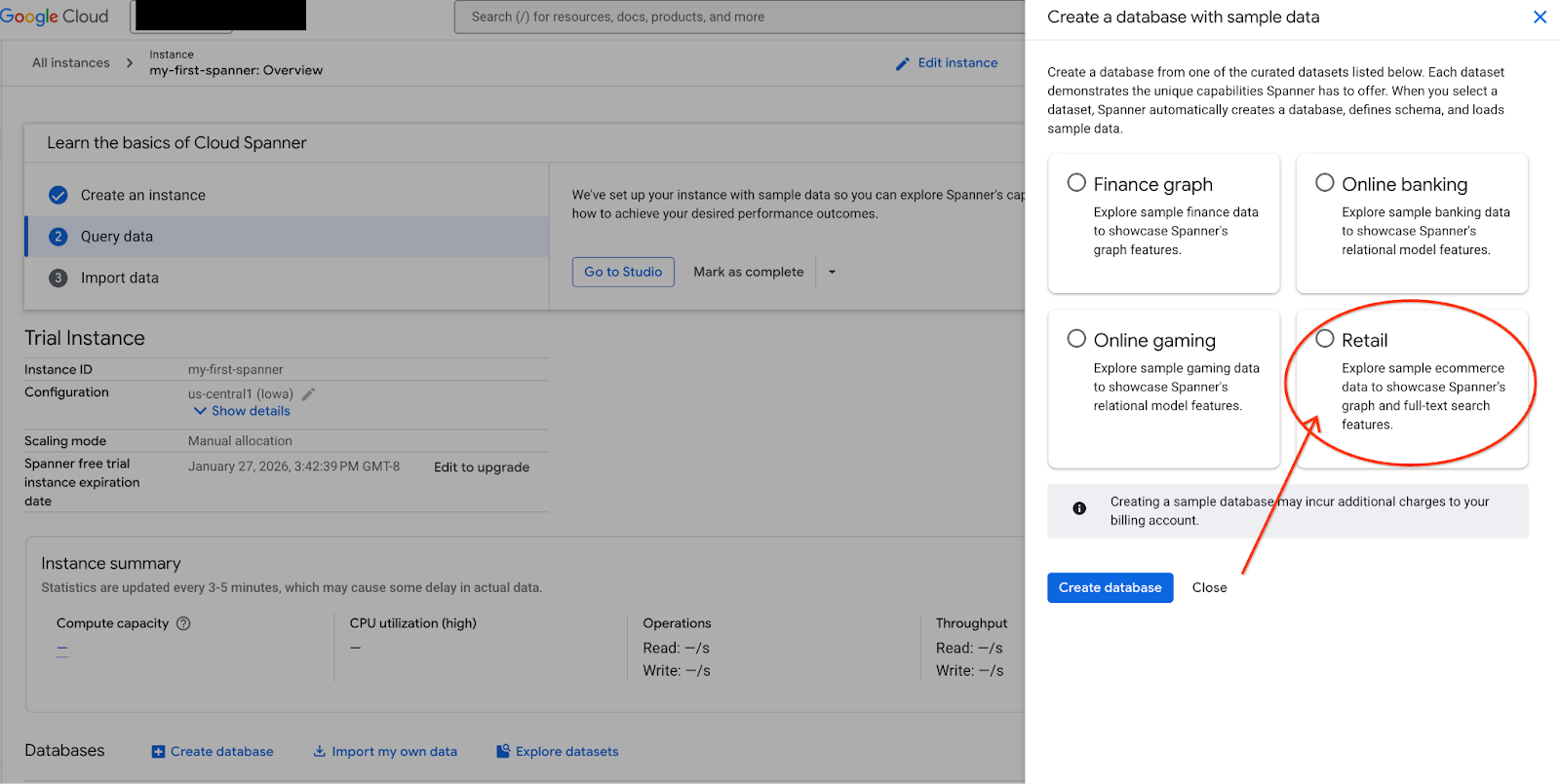
3. On the screen, select Explore Datasets. Then in the pop-up select the "Retail" option.

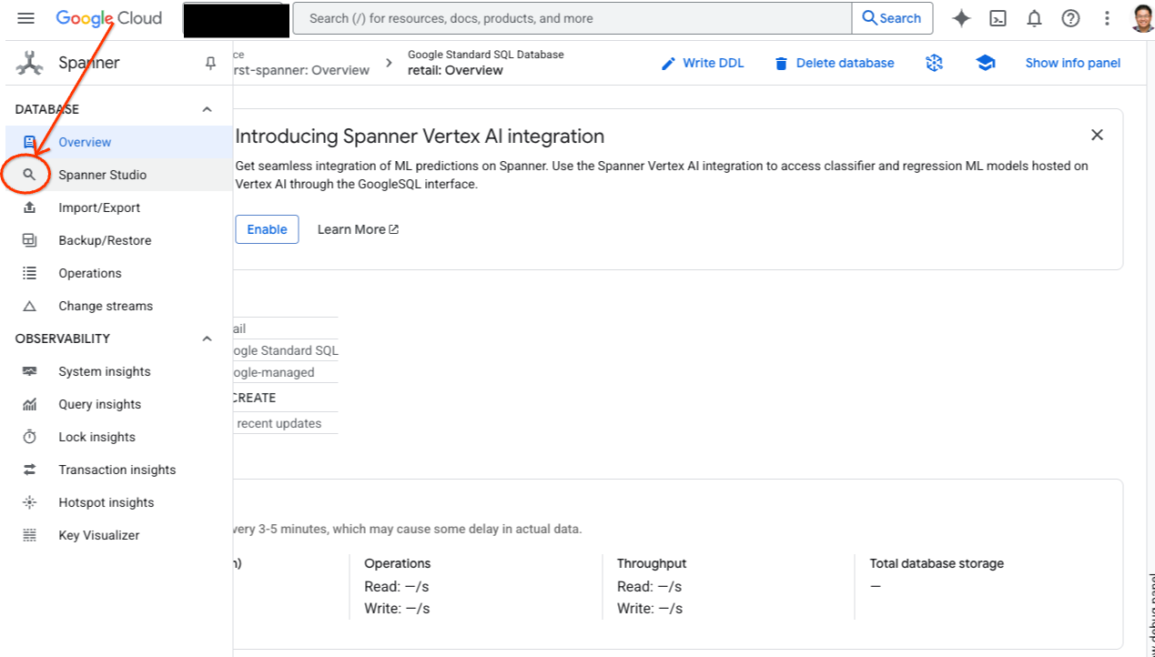
4. Navigate to Spanner Studio. Spanner Studio includes an Explorer pane that integrates with a query editor and a SQL query results table. You can run DDL, DML, and SQL statements from this one interface. You'll need to expand the menu on the side, look for the magnifying glass.

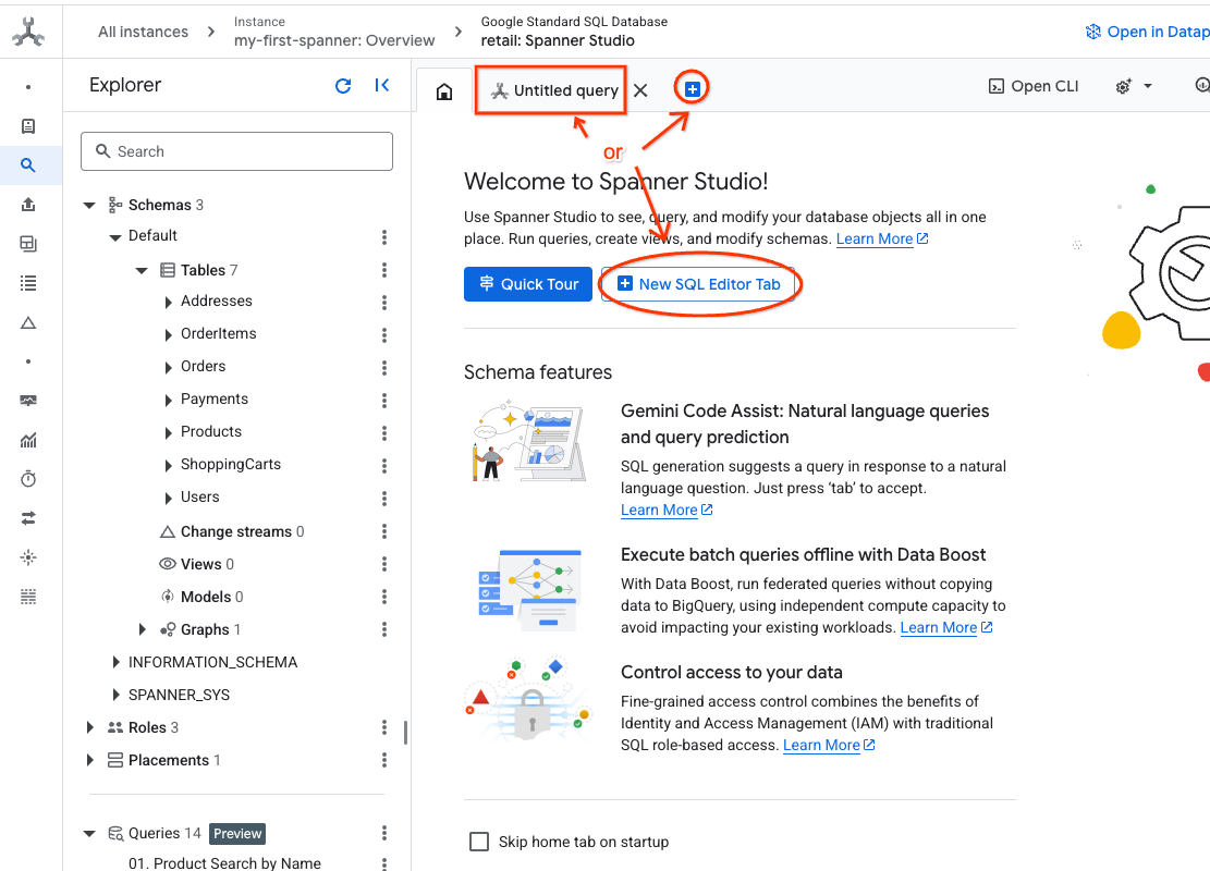
5. Read the Products table. Create a new tab or use the "Untitled query" tab already made.

SELECT *
FROM Products;

5. Step 2: Create the AI Models.

Now, let's create the remote models with Spanner objects. These SQL statements create Spanner objects that link to Vertex AI endpoints.

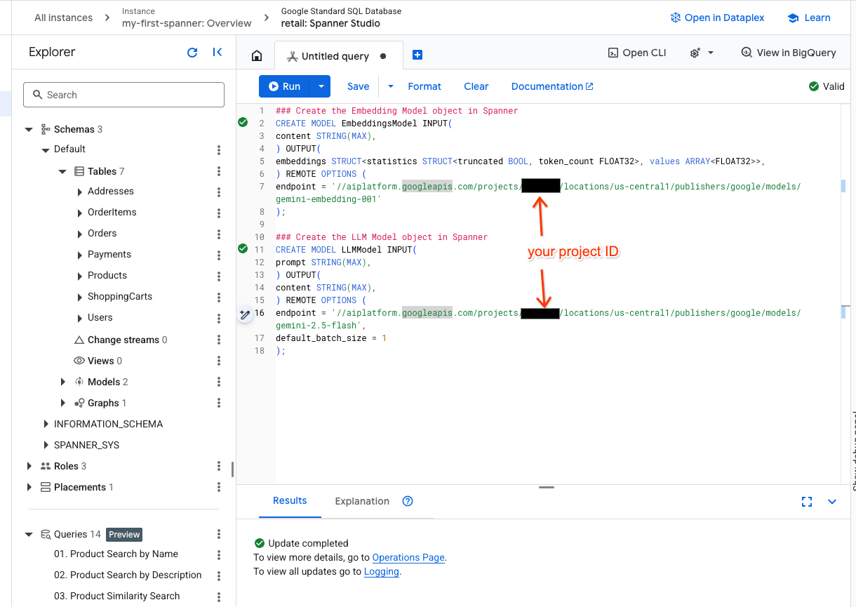
1. Open a new tab in Spanner studio and create your two models. The first is the EmbeddingsModel which will allow you to generate embeddings. The second is the LLMModel which will allow you to interact with an LLM (in our example, it's gemini-2.5-flash). Ensure you have updated the <PROJECT_ID> with your project ID.

### Create the Embedding Model object in Spanner
CREATE MODEL EmbeddingsModel INPUT(
content STRING(MAX),
) OUTPUT(
embeddings STRUCT<statistics STRUCT<truncated BOOL, token_count FLOAT32>, values ARRAY<FLOAT32>>,
) REMOTE OPTIONS (
endpoint = '//aiplatform.googleapis.com/projects/<PROJECT_ID>/locations/us-central1/publishers/google/models/text-embedding-005'
);

### Create the LLM Model object in Spanner
CREATE MODEL LLMModel INPUT(
prompt STRING(MAX),
) OUTPUT(
content STRING(MAX),
) REMOTE OPTIONS (
endpoint = '//aiplatform.googleapis.com/projects/<PROJECT_ID>/locations/us-central1/publishers/google/models/gemini-2.5-flash',
default_batch_size = 1
);

2. Note: Remember to replace PROJECT_ID with your actual $PROJECT_ID.

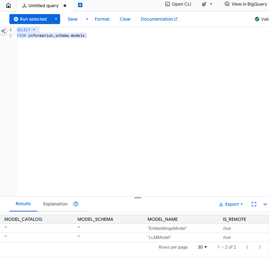
Test this step: You can verify the models were created by running the following in the SQL editor.

SELECT *
FROM information_schema.models;

6. Step 3: Generate and Store Vector Embeddings

Our Product table has text descriptions, but the AI model understands vectors (arrays of numbers). We need to add a new column to store these vectors and then populate it by running all our product descriptions through the EmbeddingsModel.

1. Create a new table to support the embeddings. First create a table that can support embeddings. We are using a different embedding model than the product table sample embeddings. You need to ensure the embeddings were generated from the same model for the vector search to work properly.

CREATE TABLE products_with_embeddings (
   ProductID INT64,
   embedding_vector ARRAY<FLOAT32>(vector_length=>768),
   embedding_text STRING(MAX)
)
PRIMARY KEY (ProductID);

2. Populate the new table with the embeddings generated from the model. We use an insert into statement for simplicity here. This will push the query results into the table you just created.

The SQL statement first grabs and concatenates all the relevant text columns we want to generate embeddings on. Then we return the relevant information, including the text we used. This is normally not necessary but we include it so you can visualize the results.

INSERT INTO products_with_embeddings (productId, embedding_text, embedding_vector)
SELECT
ProductID,
content as embedding_text,
embeddings.values as embedding_vector
FROM ML.PREDICT(
 MODEL EmbeddingsModel,
 (
   SELECT
   ProductID,
   embedding_text AS content
   FROM (
     SELECT
       ProductID,
       CONCAT(
         Category,
         " ",
         Description,
         " ",
         Name
       ) AS embedding_text
       FROM products)));

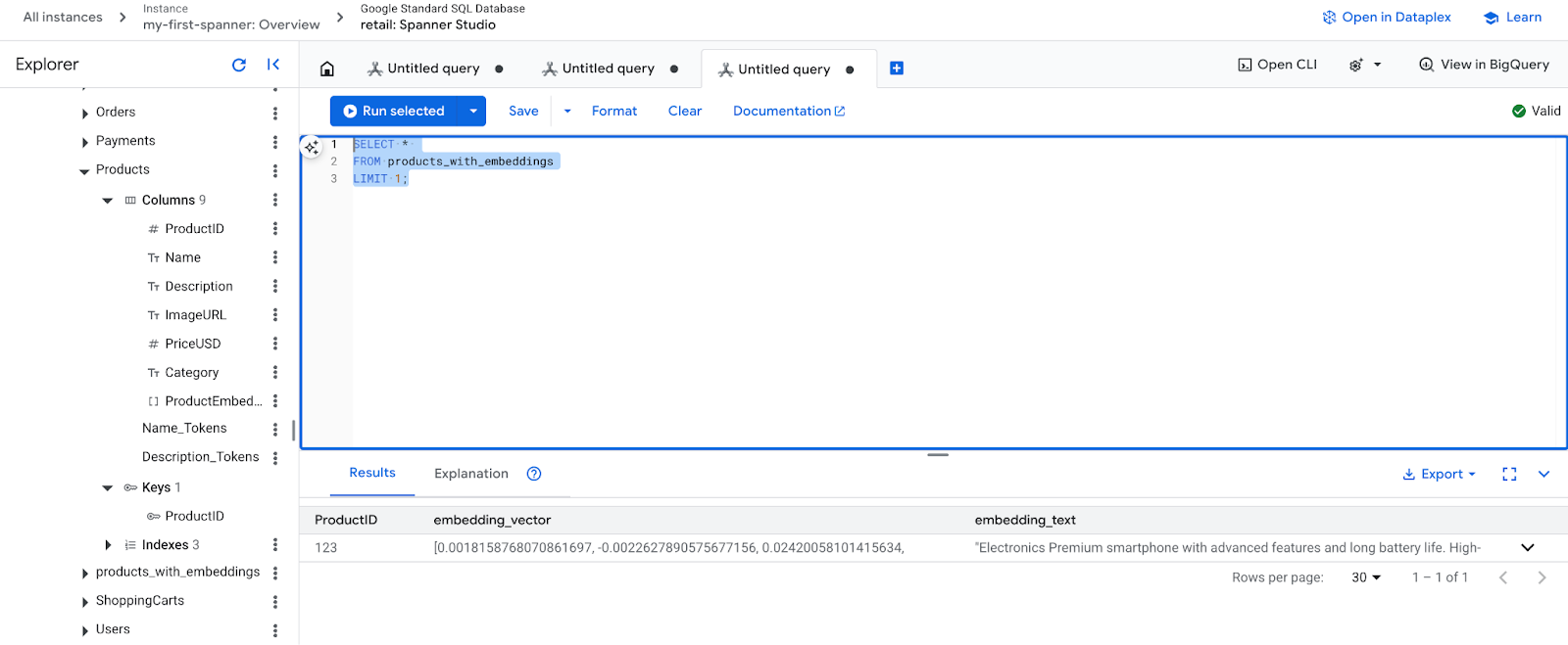
3. Check your new embeddings. You should now see the embeddings that were generated.

SELECT *
FROM products_with_embeddings
LIMIT 1;

7. Step 4: Create a Vector Index for ANN Search

To search millions of vectors instantly, we need an index. This index enables Approximate Nearest Neighbor (ANN) search, which is incredibly fast and scales horizontally.

Important: Creating a vector index is a compute-intensive operation. For a large dataset, this can take 10 minutes or more.

1. Run the following DDL query to create the index. We specify COSINE as our distance metric, which is excellent for semantic text search. Note, that the WHERE clause is actually necessary as Spanner will make it a requirement for the query.

CREATE VECTOR INDEX DescriptionEmbeddingIndex
   ON products_with_embeddings(embedding_vector)
   WHERE embedding_vector IS NOT NULL
OPTIONS (
 distance_type = 'COSINE'
);

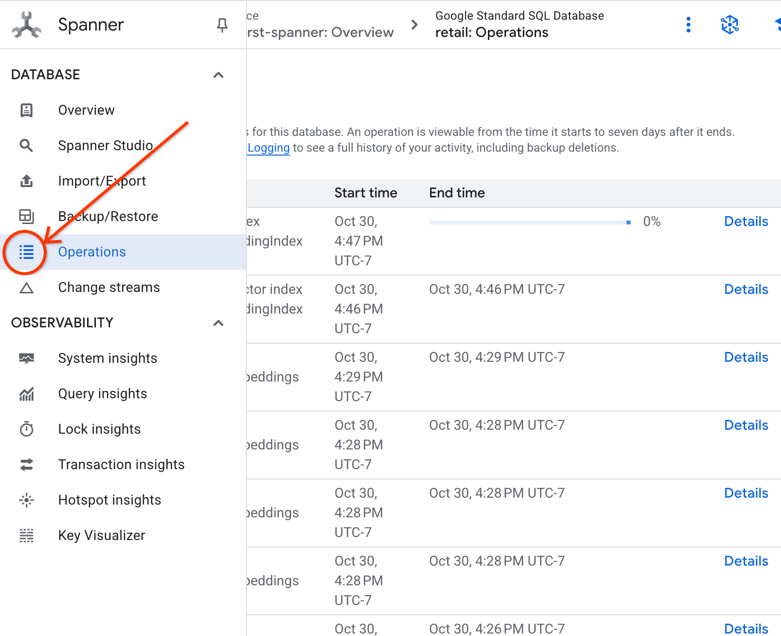
2. Check on the status of your index creation in the operations tab.

8. Step 5: Find Recommendations with K-Nearest Neighbor (KNN) Search

Now for the fun part! Let's find products that match our customer's query: "I'd like to buy a high performance keyboard. I sometimes code while I'm at the beach so it may get wet.".

We'll start with K-Nearest Neighbor (KNN) search. This is an exact search that compares our query vector to every single product vector. It's precise but can be slow on very large datasets (which is why we built an ANN index for Step 5).

This query does two things:

1. A subquery uses ML.PREDICT to get the embedding vector for our customer's query.
2. The outer query uses COSINE_DISTANCE to calculate the "distance" between the query vector and every product's embedding_vector. A smaller distance means a better match.

SELECT
    productid,
    embedding_text,
    COSINE_DISTANCE(
      embedding_vector,
      (
        SELECT embeddings.values
        FROM ML.PREDICT(
          MODEL EmbeddingsModel,
          (SELECT "I'd like to buy a high performance keyboard. I sometimes code while I'm at the beach so it may get wet." AS content)
        )
      )
    ) AS distance
FROM products_with_embeddings
WHERE embedding_vector IS NOT NULL
ORDER BY distance
LIMIT 5;

You should see a list of products, with keyboards that are water resistant at the very top.

9. Step 6: Find Recommendations with Approximate (ANN) Search

KNN is great, but for a production system with millions of products and thousands of queries per second, we need the speed of our ANN index.

Using the index requires you specify the APPROX_COSINE_DISTANCE function.

1. Get the vector embedding of your text as you did above. We cross join the results of that with the records in the products_with_embeddings table so you can use it in your APPROX_COSINE_DISTANCE function.

WITH vector_query as
(
 SELECT embeddings.values as vector
 FROM ML.PREDICT(
 MODEL EmbeddingsModel,
  (SELECT "I'd like to buy a high performance keyboard. I sometimes code while I'm at the beach so it may get wet." as content)
 )
)
SELECT
ProductID,
embedding_text,
APPROX_COSINE_DISTANCE(embedding_vector, vector, options => JSON '{\"num_leaves_to_search\": 10}') distance
FROM products_with_embeddings @{force_index=DescriptionEmbeddingIndex},
vector_query
WHERE embedding_vector IS NOT NULL
ORDER BY distance
LIMIT 5;

Expected Output: The results should be identical or very similar to the KNN query, but it executed much more efficiently by using the index. You may not notice this in the example.

10. Step 7: Use an LLM to Explain Recommendations

Just showing a list of products is good, but explaining why or why not it's a good or bad fit is great. We can use our LLMModel (Gemini) to do this.

This query nests our KNN query from Step 4 inside an ML.PREDICT call. We use CONCAT to build a prompt for the LLM, giving it:

1. A clear instruction ("Answer with ‘Yes' or ‘No' and explain why...").
2. The customer's original query.
3. The name and description of each top-matching product.

The LLM then evaluates each product against the query and provides a natural language response.

SELECT
   ProductID,
   embedding_text,
   content AS LLMResponse
FROM ML.PREDICT(
   MODEL LLMModel,
   (
     SELECT
       ProductID,
       embedding_text,
       CONCAT(
         "Answer with ‘Yes' or ‘No' and explain why: Is this a good fit for me?",
         "I'd like to buy a high performance keyboard. I sometimes code while I'm at the beach so it may get wet. \n",
         "Product Description:", embedding_text
       ) AS prompt,
     FROM products_with_embeddings
     WHERE embedding_vector IS NOT NULL
     ORDER BY COSINE_DISTANCE(
       embedding_vector,
       (
         SELECT embeddings.values
         FROM ML.PREDICT(
           MODEL EmbeddingsModel,
           (SELECT "I'd like to buy a high performance keyboard. I sometimes code while I'm at the beach so it may get wet." AS content)
         )
       )
     )
     LIMIT 5
   ),
   STRUCT(1056 AS maxOutputTokens)
);

Expected Output: You'll get a table with a new LLMResponse column. The response should be something like: "No. Here's why: * "Water-resistant" is not "waterproof." A "water-resistant" keyboard can handle splashes, light rain, or spilled"

11. Step 8: Create a Property Graph

Now for a different type of recommendation: "customers who bought this also bought..."

This is a relationship-based query. The perfect tool for this is a property graph. Spanner lets you create a graph on top of your existing tables without duplicating data.

This DDL statement defines our graph:

• Nodes: Product and User tables. The nodes are the entities you want to derive a relationship from, you want to know customers who bought your product also bought ‘XYZ' products.
• Edges: The Orders table, which connects a User (Source) to a Product (Destination) with the label "Purchased". The edges provide the relationship between a user and what they purchased.

CREATE PROPERTY GRAPH RetailGraph
 NODE TABLES (
   products_with_embeddings,
   Orders
 )
 EDGE TABLES (
   OrderItems
     SOURCE KEY (OrderID) REFERENCES Orders
     DESTINATION KEY (ProductID) REFERENCES products_with_embeddings
     LABEL Purchased
 );

12. Step 9: Combine Vector Search and Graph Queries

This is the most powerful step. We will combine AI vector search and graph queries in a single statement to find related products.

This query is read in three parts, separated by the NEXT statement, let's break it down into sections.

1. First we find the best match using vector search.
2. ML.PREDICT generates a vector embedding from the user's text query using EmbeddingsModel.
3. The query calculates the COSINE_DISTANCE between this new embedding and the stored p.embedding_vector for all products.
4. It selects and returns the single bestMatch product with the minimum distance (highest semantic similarity).
5. Next we traverse the graph in search of the relationships.

NEXT MATCH (bestMatch)<-[:Purchased]-(user:Orders)-[:Purchased]->(purchasedWith:products_with_embeddings)

1. The query traces back from bestMatch to common Orders nodes (user) and then forward to other purchasedWith products.
2. It filters out the original product and uses GROUP BY and COUNT(1) to aggregate how often items are co-purchased.
3. It returns the top 3 co-purchased products (purchasedWith) ordered by the frequency of co-occurrence.

Additionally, we find the User Order Relationship.

NEXT MATCH (bestMatch)<-[:Purchased]-(user:Orders)-[purchased:Purchased]->(purchasedWith)

1. This intermediate step executes the traversal pattern to bind the key entities: bestMatch, the connecting user:Orders node, and the purchasedWith item.
2. It specifically binds the relationship itself as purchased for data extraction in the next step.
3. This pattern ensures the context is established to fetch order-specific and product-specific details.
4. Finally, we output the results to be returned as graph nodes must be formatted before being returned as SQL results.

GRAPH RetailGraph
MATCH (p:products_with_embeddings)
WHERE p.embedding_vector IS NOT NULL
RETURN p AS bestMatch
ORDER BY COSINE_DISTANCE(
 p.embedding_vector,
 (
   SELECT embeddings.values
   FROM ML.PREDICT(
     MODEL EmbeddingsModel,
     (SELECT "I'd like to buy a high performance keyboard. I sometimes code while I'm at the beach so it may get wet." AS content)
   )
 )
)
LIMIT 1

NEXT
MATCH (bestMatch)<-[:Purchased]-(user:Orders)-[:Purchased]->(purchasedWith:products_with_embeddings)
FILTER bestMatch.productId <> purchasedWith.productId
RETURN bestMatch, purchasedWith
GROUP BY bestMatch, purchasedWith
ORDER BY COUNT(1) DESC
LIMIT 3

NEXT
MATCH (bestMatch)<-[:Purchased]-(user:Orders)-[purchased:Purchased]->(purchasedWith)
RETURN
 TO_JSON(Purchased) AS purchased,
 TO_JSON(user.OrderID) AS user,
 TO_JSON(purchasedWith.productId) AS purchasedWith;

Expected Output: You'll see JSON objects representing the top 3 co-purchased items, providing cross-sell recommendations.

13. Cleaning up

To avoid incurring charges, you can delete the resources you created.

1. Delete the Spanner Instance: Deleting the instance will delete the database as well.

gcloud spanner instances delete my-first-spanner --quiet

2. Delete the Google Cloud Project: If you created this project just for the codelab, deleting it is the easiest way to clean up.

• Go to the Manage Resources page in the Google Cloud Console.
• Select your project and click Delete.

🎉 Congratulations!

You've successfully built a sophisticated, real-time recommendation system using Spanner AI and Graph!

You've learned how to integrate Spanner with Vertex AI for embeddings and LLM generation, how to perform high-speed vector search (KNN and ANN) to find semantically relevant products, and how to use graph queries to discover product relationships. You've built a system that can not only find products but also explain recommendations and suggest related items, all from a single, scalable database.