Cloud Spanner: Graph Intelligence using Spanner Graph Algorithms

1. Case-study: Intelligent Retail

For the case-study we take a Retail Customer with a fast-growing digital marketplace. Customer's traditional data view is limited because it shows what people buy, but not how they are connected. This gap leads to missed opportunities and rising fraud. Now, they are pivoting to a Network-First philosophy to value social and logistics connections in addition to transactional data.

Core Business Challenges to address

You have four critical challenges that require understanding how customers and logistics are interconnected:

Challenge	The Problem	The Goal
Influence Gap	Broad advertising yields low ROI; currently It's not possible to identify the real trendsetters (influencers).	Identify Influencers; that are central to the community through their connection in a connected network of customers.
Logistics Resilience	The supply chain can be vulnerable (considering they operate in different geos). If one key hub fails, the entire region can potentially lose product access.	Identify Gatekeepers; those who are critical to bridge the logistics networks together.
Ghost Networks	Fraud rings use fake profiles and shared addresses to coordinate theft and inflate ratings.	Expose Isolated Islands; hyper-connected groups with no ties to the legitimate community.
Paradox of Choice	Current suggestion-/recommendation- engine is rudimentary, generic and often ignored (e.g., "Customers who bought this also bought ...").	Build Behavioral Twins; i.e. recommendations based on similar shipping patterns and social circles.

Mapping Business Challenges to a Technical Strategy (Rows → Relationships)

In a traditional database, data is stored in isolated silos: customers in one table, transactions in another, shipping in a third. While SQL is perfect for answering "Who bought what?", it struggles to answer network-based questions.

To solve these challenges, technical strategy is to shift this perspective:

• The Relational View (The "What"): Treats every customer as an isolated row. Finding a connection between a customer and a friend's purchase requires multiple complex "joins", which become exponentially slower as the network grows.
• The Graph View (The "How"): Treats relationships as first-class citizens. Instead of searching through lists, we navigate a map. We can see instantly that Customer A is connected to Customer B, who ships to Location Z.

Technical Strategy

• The customer does not intend to throw away its existing relational data.
• Instead, the intention is to create a Property Graph overlay on top of relational tables to reveal the hidden patterns of influence and risk that have been there all along.
• On Graph they intend to address their business challenges through sophisticated Graph Algorithms.

Deep diving into requirements

Solution architects come to a conclusion that business requirements and technical strategy requires a multi-model approach, and identify the following key requirements.

Technical Requirements

• Scalable Relational Foundation
• Zero ETL to build Graph representation
• Unified query language to question relational data and traverse Graph data.
• Ability to run computationally intensive Graph Algorithms without impacting the production system.
• Ability to ingest Algorithm results for down-stream analysis (preferably back to same database)

How Cloud Spanner fits those technical requirements

Cloud Spanner is chosen as the heart of this transformation. It allows the Customer to keep its rock-solid relational foundation while simultaneously unlocking deep graph insights.

It's not about choosing between a spreadsheet and a map; the intention is to build a map directly on top of the spreadsheet.

Here is a quick rundown of how Cloud Spanner addresses technical requirements and more.

Cloud Spanner Checklist towards Technical Requirements

• Zero ETL (No Data Silos): In traditional setups, you must replicate data into a separate graph database, creating lag and security risks. In Spanner, the graph lives on top of your existing tables. When a customer makes a purchase, the "edge" in your graph exists instantly.
• Interleaved Performance: Spanner's unique ability to interleave tables means a customer's profile, their friends, and their transactions are physically stored together. This turns slow, network-heavy operations into lightning-fast local lookups.
• Off-Box Analytical Isolation (Data Boost): The customer can run intensive graph algorithms (like PageRank or Community Detection) without ever slowing down the checkout process. Using Data Boost, these calculations run on independent, serverless resources, keeping the "Transaction" side of the house unaffected by the "Intelligence" exploration.
• Unified Language: Use GoogleSQL for standard reporting and ISO GQL (Graph Query Language) for relationship mining. You can even combine them in a single query to find a customer's email (SQL) and their most influential friend (GQL) simultaneously.

On top of that Cloud Spanner provides a Future proof technical architecture

Future Proofing

• Beyond Graph, Spanner provides a unified data platform where the customer can later leverage Full-Text Search, perform real-time AI inference, utilize Vector Search for hybrid recommendations - and build a true HTAP; all within a single, co-existent system.

2. Setting up Data foundation

Following the business case we now move into the implementation phase. In this section, we define our data architecture, explore the limitations of the traditional relational model, and introduce the Property Graph as our primary tool for uncovering deep insights.

Setup Cloud Spanner Enterprise Instance

Step 1: Enable Cloud Spanner API

In the Google Cloud Console, click the Menu icon on the top left of the screen for the left navigation. Scroll down and select "Spanner", or alternatively search for "Spanner"

You should now see the Cloud Spanner UI, and assuming you are using a project that hasn't enabled the Cloud Spanner API yet, you will see a dialog asking you to enable it. If you have already enabled the API, you can skip this step.

Click on "Enable" to continue:

Step 2: Create Cloud Spanner Instance

First, you will create a Cloud Spanner instance. In the UI, click on "Create a Provisioned Instance" to create a new instance.

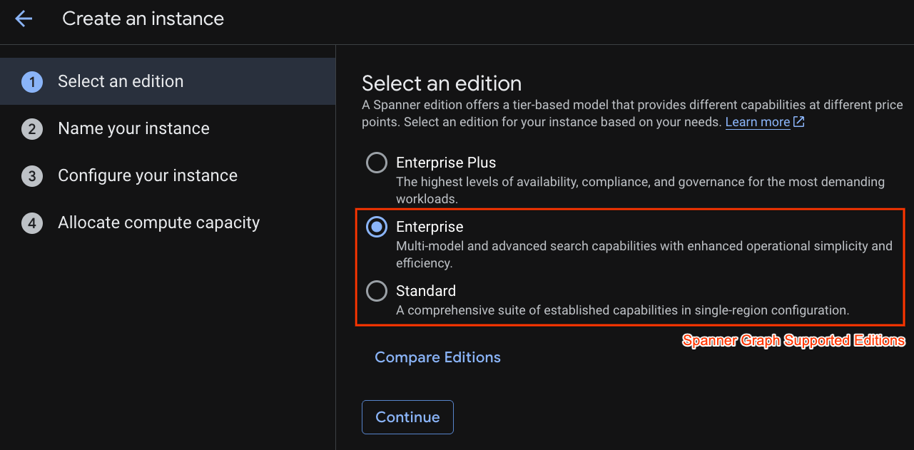
In the first step you have to select an edition. Please note that you can upgrade Edition afterwards as well. In order to use multi-model capabilities (Spanner Graph) we can go with Enterprise Edition.

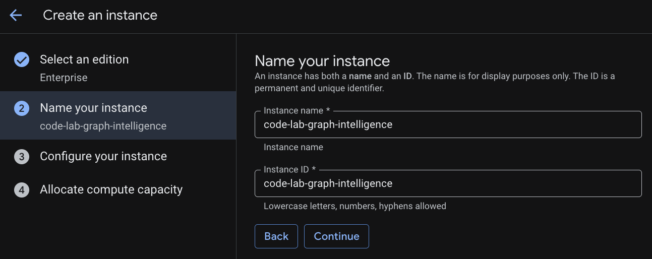
Naming your instance

Select a deployment configuration and select a regional of your choice.

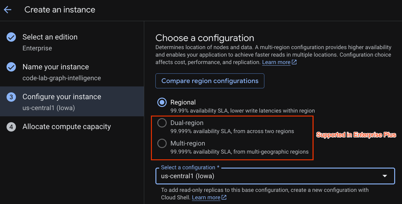
You can also compare various configuration options. For instance, the deployment configuration has at minimum 3 R/W replicas in 3 separate zones of your selected region. i.e. even if you go with a single node deployment you have 3 copies through 3 R/W replicas. In addition even with Regional deployment configuration you can further extend by having additional R/O replicas in your deployment topology.

Upon configuration of capacity, you can either start at full-node and autoscaling at nodes; or you can use a granular instance (Processing Units; 1000 PUs = 1 node). Optionally you can also set autoscaling targets of instance. For low latency workloads, we recommend 65% for regional instances and 45% for multi-region instances.

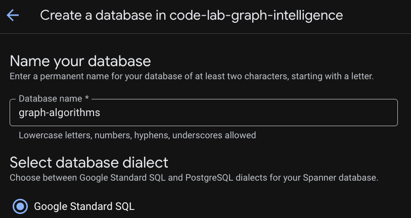
Step 3: Create a Database

Once your instance is provisioned click "Create Database" to create a database for the rest of your codelab.

Setting-up a Relational Foundation

Our journey begins with the core tables that store operational data. In Cloud Spanner, we use Interleaving to physically co-locate related data, such as a customer's friendships and transactions directly with the customer record. This ensures high-performance access and physical locality.

DDL: Creating the Tables

Copy and execute the following blocks to establish your relational schema:

-- NODE: Customer (Parent)
CREATE TABLE Customer (
  customer_id STRING(60) NOT NULL,
  customer_email STRING(32),

  -- Placeholder fields for Algorithm results
  pagerank_score FLOAT64,        
  centrality_score FLOAT64,      
  community_id INT64            
) PRIMARY KEY(customer_id);

-- EDGE: CustomerFriendship (Interleaved in Customer)
CREATE TABLE CustomerFriendship (
  customer_id STRING(60) NOT NULL,
  friend_id STRING(60) NOT NULL,
  friendship_strength FLOAT64,
  created_at TIMESTAMP,
  CONSTRAINT FK_Friend FOREIGN KEY(friend_id) REFERENCES Customer(customer_id)
) PRIMARY KEY(customer_id, friend_id),
  INTERLEAVE IN PARENT Customer ON DELETE CASCADE;

-- NODE: Product
CREATE TABLE Product (
  product_id STRING(60) NOT NULL,
  product_name STRING(32),
  unit_price FLOAT64,
  pagerank_score FLOAT64
) PRIMARY KEY(product_id);

-- NODE: Shipping
CREATE TABLE Shipping (
  shipping_id STRING(60) NOT NULL,
  city STRING(32),
  country STRING(32)
) PRIMARY KEY(shipping_id);

-- EDGE: Transactions (Interleaved in Customer)
CREATE TABLE Transactions (
  customer_id STRING(60) NOT NULL,
  row_id STRING(36) DEFAULT (GENERATE_UUID()),
  product_id STRING(60) NOT NULL,
  shipping_id STRING(60) NOT NULL,
  transaction_date TIMESTAMP,
  amount FLOAT64,
  CONSTRAINT FK_Prod FOREIGN KEY(product_id) REFERENCES Product(product_id),
  CONSTRAINT FK_Ship FOREIGN KEY(shipping_id) REFERENCES Shipping(shipping_id)
) PRIMARY KEY(customer_id, row_id),
  INTERLEAVE IN PARENT Customer ON DELETE CASCADE;

Seeding the Network

With our tables ready, we must populate them with the users, products, and connections that define The Customer's ecosystem.

-- Populate Products & Shipping
INSERT INTO Product (product_id, product_name, unit_price) VALUES
('P1', 'Smartphone Pro', 999.00), ('P2', 'Wireless Earbuds', 150.00),
('P3', 'USB-C Cable', 25.00), ('P4', '4K Monitor', 450.00),
('P5', 'Ergonomic Chair', 300.00), ('P6', 'Desk Lamp', 45.00);

INSERT INTO Shipping (shipping_id, city, country) VALUES
('S1', 'New York', 'USA'), ('S2', 'London', 'UK'), ('S3', 'Tokyo', 'Japan'),
('S4', 'San Francisco', 'USA'), ('S5', 'Berlin', 'Germany');

-- Populate Customers
INSERT INTO Customer (customer_id, customer_email) VALUES
('C1', '[e-mail]'), ('C2', '[e-mail]'), ('C3', '[e-mail]'),
('C4', '[e-mail]'), ('C5', '[e-mail]'), ('C6', '[e-mail]'),
('C7', '[e-mail]'), ('C8', '[e-mail]'), ('C9', '[e-mail]'),
('C10', '[e-mail]'), ('C11', '[e-mail]'), ('C12', '[e-mail]');

-- Populate Friendships
INSERT INTO CustomerFriendship (customer_id, friend_id, friendship_strength, created_at) VALUES
('C1', 'C2', 1.0, CURRENT_TIMESTAMP()), ('C1', 'C3', 1.0, CURRENT_TIMESTAMP()), 
('C2', 'C1', 0.8, CURRENT_TIMESTAMP()), ('C3', 'C1', 0.9, CURRENT_TIMESTAMP()),
('C3', 'C4', 0.5, CURRENT_TIMESTAMP()), ('C4', 'C5', 0.5, CURRENT_TIMESTAMP()),
('C5', 'C6', 1.0, CURRENT_TIMESTAMP()), ('C5', 'C7', 0.8, CURRENT_TIMESTAMP()), 
('C7', 'C8', 0.7, CURRENT_TIMESTAMP()), ('C8', 'C5', 0.6, CURRENT_TIMESTAMP()),
('C11', 'C1', 1.0, CURRENT_TIMESTAMP()), ('C11', 'C5', 1.0, CURRENT_TIMESTAMP()), 
('C11', 'C7', 1.0, CURRENT_TIMESTAMP()), ('C11', 'C12', 0.5, CURRENT_TIMESTAMP()),
('C1', 'C11', 0.9, CURRENT_TIMESTAMP()), ('C5', 'C11', 0.9, CURRENT_TIMESTAMP()),
('C9', 'C10', 1.0, CURRENT_TIMESTAMP()), ('C10', 'C9', 1.0, CURRENT_TIMESTAMP());

-- Populate Transactions
INSERT INTO Transactions (customer_id, product_id, shipping_id, amount, transaction_date) VALUES
('C1', 'P1', 'S1', 999.00, CURRENT_TIMESTAMP()), ('C2', 'P1', 'S1', 999.00, CURRENT_TIMESTAMP()),
('C11', 'P4', 'S4', 450.00, CURRENT_TIMESTAMP()), ('C11', 'P5', 'S4', 300.00, CURRENT_TIMESTAMP()),
('C7', 'P5', 'S5', 300.00, CURRENT_TIMESTAMP()), ('C8', 'P6', 'S5', 45.00, CURRENT_TIMESTAMP()),
('C9', 'P1', 'S1', 999.00, CURRENT_TIMESTAMP()), ('C10', 'P1', 'S1', 999.00, CURRENT_TIMESTAMP());

Relational Challenge

Before we introduce the graph, let's see how traditional SQL handles The Customer's challenges. Run this query to find "Social Spenders"customers who spend significantly and have several friends.

SELECT 
    c.customer_id, 
    c.customer_email,
    SUM(t.amount) AS total_spent,
    COUNT(DISTINCT f.friend_id) AS friend_count
FROM Customer AS c
LEFT JOIN Transactions AS t ON c.customer_id = t.customer_id
LEFT JOIN CustomerFriendship AS f ON c.customer_id = f.customer_id
GROUP BY c.customer_id, c.customer_email
HAVING total_spent > 500
ORDER BY total_spent DESC;

The Limitations of the Relational Approach

SQL suffers from several critical drawbacks in a "Network-First" business:

• The "Join" Penalty: To find what a friend-of-a-friend bought, you must join multiple large tables. In SQL, this would require joining four tables (Customer → Friendship → Transactions → Product), which becomes computationally expensive as connections grow.
• One-Hop Blindness: Relational queries are excellent at finding direct links (1-hop), but they struggle with transitive relationships. For example, identifying a fraud ring where Customer A and Customer B share an address, but Customer B is only connected to Customer C via a social link, requires complex recursive joins in SQL.
• Readability: As The Customer asks deeper questions about connectivity, the SQL queries become increasingly dense and difficult to maintain.

Overcoming Relational Challenges through a Property Graph

To overcome these limits, we define a Property Graph. This creates an "overlay" that allows us to treat relationships as first-class citizens without moving our data out of Spanner.

DDL: Creating the Property Graph

This DDL defines our Nodes (Entities) and Edges (Relationships). In this example we are following a schematized graph, however Spanner Graph allows allows modeling schemaless graphs to enable flexible, rapid iterative development and to handle evolving data models without constant DDL (Data Definition Language) changes.

CREATE OR REPLACE PROPERTY GRAPH RetailTransactionGraph
NODE TABLES (
  Customer KEY (customer_id),
  Product KEY (product_id),
  Shipping KEY (shipping_id)
)
EDGE TABLES (
  CustomerFriendship AS IsFriendsWith
    SOURCE KEY (customer_id) REFERENCES Customer (customer_id)
    DESTINATION KEY (friend_id) REFERENCES Customer (customer_id)
    LABEL IsFriendsWith,
    
  Transactions AS Purchased
    SOURCE KEY (customer_id) REFERENCES Customer (customer_id)
    DESTINATION KEY (product_id) REFERENCES Product (product_id)
    LABEL Purchased,

  Transactions AS LivesAt
    SOURCE KEY (customer_id) REFERENCES Customer (customer_id)
    DESTINATION KEY (shipping_id) REFERENCES Shipping (shipping_id)
    LABEL LivesAt
);

Navigating the Graph with GQL

Now that our graph is defined, we can use Graph Query Language (GQL) to perform multi-hop traversals with a simple, readable syntax.

Exploration 1: Collaborative Discovery

This query traverses the graph to find products purchased by your friends and serves as the foundation of a recommendation engine.

GRAPH RetailTransactionGraph
MATCH (me:Customer)-[:IsFriendsWith]->(friend:Customer)-[:Purchased]->(p:Product)
WHERE me.customer_id = 'C1'
RETURN 
    me.customer_id AS my_id, 
    friend.customer_id AS friend_id, 
    p.product_name AS recommendation

Note: The syntax (node)-[:EDGE]->(node) visually represents the traversal. In GQL, this multi-hop jump is a single readable path rather than a four-table join.

Exploration 2: The Hybrid Query (Relational + Graph)

Spanner allows you to embed GQL patterns inside a standard SQL FROM clause using the GRAPH_TABLE function. This query finds customers who live at the same location as their friendsa "diamond" pattern match.

SELECT *
FROM GRAPH_TABLE(RetailTransactionGraph
  MATCH (a:Customer)-[:IsFriendsWith]-(b:Customer),
        (a)-[:LivesAt]->(loc:Shipping),
        (b)-[:LivesAt]->(loc)
  RETURN a.customer_id AS user_A, b.customer_id AS user_B, loc.city
)

Visualizing The Customer's Connections

Finally, let's use GQL to visualize our network. These queries wrap the path results in SAFE_TO_JSON, allowing visualizers to draw the nodes and lines.

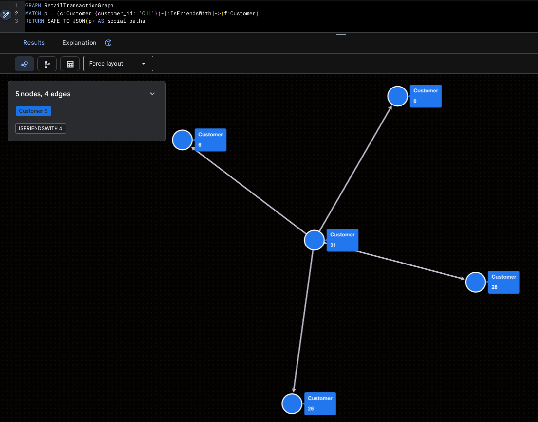
Visualizing the Super-Influencer

This highlights Mallory (C11) and her direct social reach.

GRAPH RetailTransactionGraph
MATCH p = (c:Customer {customer_id: 'C11'})-[:IsFriendsWith]->(f:Customer)
RETURN SAFE_TO_JSON(p) AS social_paths

Visualizing Potential Fraud Patterns

This query roots out the "Isolated Cluster" (Ivan & Judy) to see where their products are being shipped.

GRAPH RetailTransactionGraph
MATCH p = (c:Customer)-[:Purchased]->(prod:Product),
      q = (c)-[:LivesAt]->(loc:Shipping)
WHERE c.customer_id IN ('C9', 'C10')
RETURN SAFE_TO_JSON(p) AS purchase_path, SAFE_TO_JSON(q) AS shipping_path

💡 What did we discover? We can now see that Ivan and Judy ship to the same location, yet they are socially disconnected from the "Mainland" of The Customer. In our next section, we will use Graph Algorithms to mathematically prove and automate the detection of these patterns.

3. Introduction to Spanner Graph Algorithms

To prepare for our deep dive into Graph Intelligence, this section outlines the technical architecture and foundational rules of Cloud Spanner Graph Algorithms. Understanding these principles is key to moving from simple traversals to petabyte-scale relationship analysis.

The Algorithm Portfolio

Cloud Spanner currently supports 14 industry-standard graph algorithms, categorized into four functional groups to solve diverse business problems:

Category	Supported Algorithms	Business Use Case
Centrality	PageRank, Personalized PageRank, Betweenness, Closeness	Identify influencers, hubs, and bottlenecks.
Community	WCC, Label Propagation, Clique Finding, Correlation Clustering	Detect fraud rings, social communities, and silos.
Similarity	Jaccard, Cosine, Common Neighbors, Total Neighbors	Power recommendation engines and entity resolution.
Path Finding	Set-to-set Shortest Path, GA Path helpers	Optimize logistics and traversal proximity.

Crucial Schema & Query Considerations

In order to ensure efficient Graph algorithms execution, Spanner Graph needs to adhere to these rules:

Requirement 1. Physical Data Locality (Interleaving)

The most critical requirement for high-performance graph traversal is Interleaving. This ensures that edge data is physically stored on the same server split as the source node, minimizing network latency during algorithm execution.

• The Rule: Edge tables MUST be interleaved in their source node tables.
• Forward Traversal: Interleaving the edge table into the source node table ensures cache locality for outgoing links.
• Reverse Traversal: For efficient "incoming" link analysis, use Foreign Keys to automatically create backing indexes, or create a secondary index interleaved in the destination table.

⚠️ Caution: Failure to interleave edge tables correctly will prevent the use of graph algorithms and significantly degrade standard traversal performance. Please refer to Spanner Schema for Graph Traversal Best Practices.

Requirement 2. Unique Labeling Requirements

Every table participating in the property graph must have a unique identity. Algorithms rely on these labels to correctly identify and load the subgraphs they need to analyze.

• The Rule: Each input table must have a uniquely identifying label within the property graph.
• The Conflict: You cannot map a single label to multiple tables if you intend to run algorithms on them.

Logic	Example	Result
❌ Bad	NODE TABLES (Person LABEL Entity, Account LABEL Entity)	Invalid: The algorithm cannot distinguish between a Person and an Account.
✅ Good	NODE TABLES (Person LABEL Customer, Account LABEL Account)	Valid: Each entity has a distinct, unique label.

Requirement 3. Algorithm Query Structure (The MATCH Clause)

When calling an algorithm, the MATCH clause follows more restrictive rules than standard GQL queries to ensure the execution engine can optimize the analytical pipeline.

• One Pattern Per MATCH: Each MATCH statement can only name one variable.
• No Multi-Node Patterns: You cannot define a relationship pattern (e.g., (a)-[e]->(b)) directly inside a MATCH clause intended for an algorithm call.
• Literal Filters Only: While you can use WHERE clauses to filter nodes (e.g., WHERE a.id > 400), query parameters (@param) are not currently supported in graph algorithm queries.

Requirement 4. The RETURN Clause (Scalars Only)

The RETURN clause in an algorithm query acts as the bridge between the graph world and the relational world. It is strictly limited to returning scalars and constants.

• The Rule: You cannot return a "Graph Element" (the raw node or edge object).
• No Transformations: You cannot perform mathematical operations or apply functions to the properties being returned within the RETURN statement itself.

RETURN Clause Restrictions

✅ Supported	❌ Not Supported
RETURN node.id, score	RETURN node, score (Cannot return Graph Element)
RETURN PATH_LENGTH(p)	RETURN node.id + 1, score (No operations on properties)
RETURN node.name	RETURN JSON_OBJECT(node.id, score) (No functions)

Requirement 5. Data Integrity: Eliminating Dangling Edges

A "Dangling Edge" occurs when an edge points to a destination node that does not exist in the graph. This causes algorithm execution to fail because the graph structure is inconsistent.

• The Solution: Use referential constraints (Foreign Keys) and ON DELETE CASCADE to maintain graph integrity.
• Query Safety: When calling an algorithm, you must ensure that all nodes referred to by the selected edges are also included in the node_labels argument.

💡 Note: Maintaining strict referential integrity not only prevents "Dangling Edge" errors but also improves overall query speed by allowing the optimizer to make assumptions about the graph's structure.

Persistent Output: EXPORT DATA Options

Because graph algorithms are compute-intensive, they are executed in Scale-up execution mode using the EXPORT DATA statement. This leverages Data Boost, using independent serverless compute resources to prevent any lag on your production transactions.

Option 1: Persist back to Cloud Spanner

To push results directly back into your tables (e.g., saving a PageRank score), use format = ‘CLOUD_SPANNER'.

• update_ignore_all: Only updates rows for keys that already exist in the target table.
• upsert_ignore_all: Updates existing rows or inserts new rows if the keys are missing.

EXPORT DATA OPTIONS (
  format = 'CLOUD_SPANNER',
  table = 'Customer',
  write_mode = 'update_ignore_all'
) AS
GRAPH RetailTransactionGraph
CALL PageRank(...)
RETURN node.customer_id, score;

Option 2: Persist results to Google Cloud Storage (GCS)

For large-scale offline analysis, you can export to GCS in CSV, Avro, or Parquet formats.

• Wildcards: Use uri => 'gs://bucket/file_*.csv' to enable sharded output, allowing Spanner to write to multiple files in parallel for massive datasets.
• Compression: Supports GZIP, SNAPPY, and ZSTD to optimize storage costs.

EXPORT DATA OPTIONS (
  uri = 'gs://bucket/pagerank_*.csv',
  format = 'CSV',
  overwrite = true
) AS
GRAPH RetailTransactionGraph
CALL PageRank(...)
RETURN node.customer_id, score;

⚠️ Critical Notes & Cautions

No Query Parameters: Currently, graph algorithm queries do not support query parameters (@param). All arguments (like damping factors or node labels) must be literal values in the query string.

Scalar Return Operations: You cannot perform mathematical operations or apply functions directly within the RETURN clause of an algorithm call (e.g., RETURN node.id + 1 is not supported).

Serverless Billing: Spanner Graph algorithms follow a serverless billing model. You are only billed for the Serverless Processing Units (SPUs) consumed during the specific execution of the algorithm.

4. Challenge 1: Influence Gap (PageRank)

In this section, we tackle The Customer's first business hurdle: the "Influence Gap." We will move from a basic "popularity contest" to a mathematically driven map of true social influence.

Problem Statement: The Customer's marketing team has a problem. They are spending millions on broad advertising with shrinking returns because they cannot identify the "Social Superstars", those rare individuals whose endorsements ripple through the entire network.

To solve this, we need to rank our customers by Influence.

Relational Solution (Degree Centrality)

In a standard database, the easiest way to find an influencer is to simply count their followers (a metric known as Degree Centrality).

Run this query to find most "popular" users:

SELECT 
    friend_id AS customer_id, 
    COUNT(*) AS follower_count
FROM CustomerFriendship
GROUP BY friend_id
ORDER BY follower_count DESC;

customer_id	follower_count
C1	3
C5	3
C11	2
C7	2
C10	1
C12	1
C2	1
C3	1
C4	1
C6	1
C8	1
C9	1

⚠️ Quantity vs. Quality

This SQL approach treats every follower as equal . It cannot distinguish between a user followed by 100 inactive accounts and a user followed by 10 high-value "VIP" influencers .

In our data, Alice (C1) and Eve (C5) both have the same follower count. Relational SQL tells us they are identical, but as we are about to see, the graph tells a very different story.

Graph Intelligence (PageRank)

To find the real leaders, we use PageRank. This is the same algorithm that powered early web search; it measures a node's importance based on the quantity AND the quality of incoming links .

• Random Surfer Model: PageRank simulates a user moving through the graph. The Damping Factor (default 0.85) represents the probability they continue clicking; otherwise, they "teleport" to a random node .
• Power of Association: A link from an influential person (like Mallory) is worth significantly more than a link from someone with no other connections.

We will execute PageRank Algorithm and use EXPORT DATA to save the results directly into our pagerank_score column .

EXPORT DATA OPTIONS (
  format = 'CLOUD_SPANNER',
  table = 'Customer',
  write_mode = 'update_ignore_all' -- Updates existing rows
) AS
GRAPH RetailTransactionGraph
CALL PageRank(
  node_labels => ['Customer'],      -- Target our Customer nodes 
  edge_labels => ['IsFriendsWith'], -- Analyze the social ties
  damping_factor => 0.85,           -- Standard decay
  max_iterations => 10              -- Higher iterations for better precision
)
YIELD node, score               
RETURN node.customer_id, score as pagerank_score;

"Influence" Dashboard using PageRank

Now that the scores are persisted, let's compare our "Before" (Follower Count) with our "After" (PageRank Score).

-- Note that Higher PageRank score means more influential
SELECT 
    c.customer_id, 
    c.customer_email,
    count_query.follower_count,
    c.pagerank_score
FROM Customer c
JOIN (
    SELECT friend_id, COUNT(*) AS follower_count 
    FROM CustomerFriendship GROUP BY friend_id
) AS count_query ON c.customer_id = count_query.friend_id
ORDER BY c.pagerank_score DESC;

customer_id	customer_email	follower_count	pagerank_score
C5	[e-mail]	3	0.158392489
C10	[e-mail]	1	0.1093561724
C9	[e-mail]	1	0.1093561724
C1	[e-mail]	3	0.1000888124
C8	[e-mail]	1	0.09759821743
C11	[e-mail]	2	0.09466411918
C7	[e-mail]	2	0.08016719669
C6	[e-mail]	1	0.06022448093
C2	[e-mail]	1	0.0547891818
C3	[e-mail]	1	0.0547891818
C12	[e-mail]	1	0.04029225558
C4	[e-mail]	1	0.04028172791

Analysis: Who are the Real Superstars?

By analyzing the output, you can now make three critical marketing discoveries:

💡 The Hidden Gem (Eve, C5): While Eve and Alice have the same number of followers, Eve's PageRank is significantly higher . This is because Eve is part of a "reciprocal loop"her friends are also influential.

💡 The Loop Effect (Ivan & Judy, C9/C10): Ivan and Judy have only one follower each, yet their PageRank is higher than Alice's. Because they follow only each other, they pass their importance back and forth in an isolated loop.

⚠️ We need to investigate the Loop Effect in Fraud Ring section.

💡 The Quality Over Quantity Win (Mallory, C11): Mallory has fewer followers than Alice but a high score relative to her reach. PageRank recognizes that Mallory is connected to the right people, making her a high-efficiency target for brand ambassadorship.

Business Takeaway

Instead of blindly emailing everyone with more than five followers, The Customer's marketing team can now focus exclusively on those with the highest pagerank_score. These individuals are the true "Social Superstars" capable of driving systemic virality across the entire marketplace.

Now lets try to identify the Gatekeepers that keep The Customer's logistics network running.

5. Challenge 2: Logistic Resilience (BetweennessCentrality)

In this section, we address Logistics Resilience. We will move beyond measuring success by "volume" to identifying the vital "gatekeepers" that keep the network connected.

⚠️ If a key hub or a specific "bridge" connection fails, entire subnetwork can possibly lose access to products. We can keep track of that through transaction volume, but its possible and important to surface critical nodes might actually be "hidden" in the network structure.

Relational Solution (Volume-Based Analysis)

In a standard relational setup, a "critical" shipping hub is typically defined as the one processing the most orders or generating the most revenue.

Run this query to identify "top" hubs by transaction count:

-- Identify "Critical" hubs by transaction volume
SELECT 
    s.city, 
    s.country, 
    COUNT(t.row_id) AS transaction_count,
    SUM(t.amount) AS total_revenue
FROM Shipping s
JOIN Transactions t ON s.shipping_id = t.shipping_id
GROUP BY s.city, s.country
ORDER BY transaction_count DESC;

city	country	transaction_count	total_revenue
New York	USA	4	3996
Berlin	Germany	2	345
San Francisco	USA	2	750

⚠️ Volume != Criticality

This approach creates a blind spot. A small regional hub (like Berlin, S5) might only process a few orders, but if it is the only path to an entire region, its failure is far more catastrophic than a high-volume hub (like New York, S1) that has multiple redundant alternatives. SQL aggregates data but cannot "see" the physical structure of the paths between users.

To address the mismatch, we will use both IsFriendsWith and LivesAt edges. This transforms our analysis from a transaction hub to also include social check.

Graph Intelligence (Betweenness Centrality)

To find the real bottlenecks, we use Betweenness Centrality. This algorithm quantifies how often a node acts as a "bridge" along the shortest paths between all other pairs of nodes in the graph. High scores pinpoint the true gatekeepers who control the flow of goods or information.

⚠️ Logistics Resiliance

Logistics stability is tied to social trust. We analyze the graph using both IsFriendsWith (social) and LivesAt (logistics) edges because a "Systemic Gatekeeper" is an entity that connects disparate social groups to physical shipping hubs. If these "bridge" nodes fail, both the social flow of recommendations and the physical flow of goods are disrupted.

Running & Persisting Betweenness Centrality

We will execute the algorithm using EXPORT DATA and save the scores into the centrality_score column. We use Data Boost to ensure this heavy "shortest path" calculation has near-zero impact on The Customer's live operations.

EXPORT DATA OPTIONS (
  format = 'CLOUD_SPANNER',
  table = 'Customer',
  write_mode = 'update_ignore_all' 
) AS
GRAPH RetailTransactionGraph
CALL BetweennessCentrality(
  -- We include both Customer and Shipping nodes for a full ecosystem view
  node_labels => ['Customer', 'Shipping'], 
  -- We factor in social ties AND physical shipping locations
  edge_labels => ['IsFriendsWith', 'LivesAt'], 
  num_source_nodes => 100
)
YIELD node, score
-- We only persist scores for Customers; Shipping node results are safely ignored
RETURN node.customer_id, score as centrality_score;

Analysis: Identifying the "Hidden Bottlenecks"

Now, we compare our structural risk (centrality_score) with our transactional volume (order_count) to find the nodes that The Customer's leadership should worry about.

SELECT 
    c.customer_id, 
    c.customer_email,
    c.centrality_score,
    count_query.order_count
FROM Customer c
LEFT JOIN (
    SELECT customer_id, COUNT(*) AS order_count 
    FROM Transactions GROUP BY customer_id
) AS count_query ON c.customer_id = count_query.customer_id
ORDER BY c.centrality_score DESC;

customer_id	customer_email	centrality_score	order_count
C11	[e-mail]	44.5	2
C1	[e-mail]	35.5	1
C5	[e-mail]	35.5
C7	[e-mail]	12	1
C8	[e-mail]	10	1
C3	[e-mail]	6
C4	[e-mail]	3.5
C10	[e-mail]	0	1
C12	[e-mail]	0
C2	[e-mail]	0	1
C6	[e-mail]	0
C9	[e-mail]	0	1

By analyzing these results, The Customer makes three startling discoveries:

💡 The Super-Gatekeeper (Mallory, C11): Mallory holds the highest risk score. Structural analysis identifies her as the primary Global Anchor, that bridges disparate social communities with the physical logistics infrastructure. If her account or associated hub is compromised, it disrupts the flow between more pairs of customers and shipping hubs than any other node..

💡 The Community Gateways (Alice, C1 & Eve, C5): Alice and Eve are perfectly tied with an identical risk score of 35.5. They function as mirrored nodes, each serving as an exit point for their respective social clusters to access the global network.

💡 Structural vs. Transactional Value: Standard SQL reporting prioritizes high-volume spenders, leaving structural bottlenecks completely invisible.

Business Takeaway

The Customer can now prioritize its logistics redundancy and security protocols based on multi-modal structural risk. Mallory, Alice, and Eve are the gatekeepers who must be protected to ensure the stability of the logistical network.

Now let's try to isolate fraud islands.

6. Challenge 3: Ghost Networks (WCC)

In this section, we tackle the third business hurdle: The "Ghost Networks." We will move from simple "hotspot" detection to uncovering sophisticated, isolated fraud rings using community detection. The challenge here is that bad actors create fake profiles that share shipping addresses or interact in closed loops to coordinate thefts and inflate product ratings. But they are often completely isolated from the legitimate The Customer community.

To solve this, we need to expose these "Isolated Islands."

Relational Solution (Shared Identifier Search)

Without graph algorithms, the standard way to find fraud is to look for "hotspots" of shared data, such as multiple customers shipping to the exact same address .

Run this query to find customers linked by a shared shipping location:

SELECT 
    shipping_id, 
    COUNT(DISTINCT customer_id) AS customer_count,
    ARRAY_AGG(customer_id) AS linked_customers
FROM Transactions
GROUP BY shipping_id
HAVING customer_count > 1;

shipping_id	customer_count	linked_customers
S1	4	["C1","C10","C2","C9"]
S5	2	["C7","C8"]

⚠️ Transitive Blindness

This query only finds direct, "1-hop" links. If Customer A and Customer B share an address, and Customer B is "Friends" with Customer C (who uses a different address), standard SQL cannot easily link Customer A to Customer C as part of the same ring.

To find the fraud networks, we need to understand transitive reachability.

Graph Intelligence (Weakly Connected Components)

To find the full extent of these rings, we use Weakly Connected Components (WCC). WCC is a clustering algorithm that identifies sets of nodes where a path exists between any two nodes, regardless of the direction of the edges.

• Reachability Zones: It effectively carves the graph into "islands" or "reachability zones".
• Unified Entity View: By analyzing both social ties (IsFriendsWith) and logistics ties (LivesAt) simultaneously, we can group fragmented profiles into a single, unified "Impact Cluster".

Running & Persisting WCC

We will execute the WCC algorithm and save the results into the community_id column. We use Data Boost to ensure this deep reachability analysis happens on independent compute resources.

EXPORT DATA OPTIONS (
  format = 'CLOUD_SPANNER',
  table = 'Customer',
  write_mode = 'update_ignore_all' 
) AS
GRAPH RetailTransactionGraph
CALL WeaklyConnectedComponents(
  node_labels => ['Customer', 'Shipping'], 
  edge_labels => ['IsFriendsWith', 'LivesAt']
)
YIELD node, cluster
-- node.customer_id will be NULL for Shipping nodes; 
-- EXPORT DATA will safely ignore those rows.
RETURN node.customer_id, cluster AS community_id;

Analysis: Fraud Rings

Now, let's run a validation query to see our isolated communities. Legitimate users typically belong to the "Mainland," while fraudsters are often stranded on small "Islands".

SELECT 
    community_id, 
    COUNT(*) AS member_count,
    ARRAY_AGG(customer_email) AS members
FROM Customer
GROUP BY community_id
ORDER BY member_count ASC;

community_id	member_count	members
1	2	["[e-mail]","[e-mail]"]
0	10	["[e-mail]","[e-mail]","[e-mail]","[e-mail]","[e-mail]","[e-mail]","[e-mail]","[e-mail]","[e-mail]","[e-mail]"]

By running this community detection, you can identify a critical anomaly:

💡 Community 1: The Isolated "Fraud Ring": This group contains only two members: [e-mail] (C10) and [e-mail] (C9).

WCC has flagged these two as being completely isolated from the other 10 customers. Even though they might have high PageRank scores (because they follow each other in a loop), they have zero paths leading to the rest of The Customer's network.

💡 Guilt by Association: If Judy is caught with a stolen credit card, the system now knows that Ivan is part of her specific Cluster/Community and should be immediately flagged for review

Business Takeaway

The Customer can now automate its security responses. Instead of manually chasing individual accounts, they can write a simple rule: "If a community_id has fewer than three members, flag the entire group for manual KYC (Know Your Customer) review"

.

With our fraud rings exposed, we can solve the "Behavioral Twin."

7. Challenge 4: Behavioral Twin (JaccardSimilarity)

In this final challenge, we address the fourth hurdle: the "Paradox of Choice"/"Behavioral Twin". We will move from generic "frequently bought together" lists to hyper-personalized recommendations based on behavioral "fingerprints."

The Customer's current product suggestions are too generic. Recommending a popular USB cable to every customer is safe, but it isn't personal. The Customer wants to build "Behavioral Twin" recommendations identifying customers who share unique shipping patterns and social circles to suggest products with high-precision matching.

To solve this, we need to calculate the "Proximity" between users.

Relational Solution (Absolute Overlap)

In a standard relational setup, you might look for people who ship to the same locations as a reference user, like Alice (C1).

Run this query to find Alice's geographic neighbors:

SELECT 
    t2.customer_id AS similar_customer,
    COUNT(DISTINCT t1.shipping_id) AS shared_locations
FROM Transactions t1
JOIN Transactions t2 ON t1.shipping_id = t2.shipping_id
WHERE t1.customer_id = 'C1' AND t2.customer_id != 'C1'
GROUP BY similar_customer
ORDER BY shared_locations DESC;

similar_customer	shared_locations
C2	1
C10	1
C9	1

⚠️ "Union" Problem

This query tells you who shares a location, but it doesn't tell you how uniquely similar they are. If Alice ships to 100 places and Ivan only ships to 1, they are less "similar" than two people who both ship only to the same single location. SQL struggles to calculate this ratio (Intersection vs. Union) efficiently.

Graph Intelligence (Jaccard Similarity)

To find true behavioral twins, we use Jaccard Similarity. This algorithm calculates a normalized score (0.0 to 1.0) by dividing the number of shared neighbors (Intersection) by the total number of unique neighbors (Union).

Here a "Behavioral Twin" is defined by more than just a shared shipping address. By analyzing the intersection of physical footprints (LivesAt) and social ecosystems (IsFriendsWith), we can identify users who share the same lifestyle and community influence, leading to far more accurate product recommendations.

First create a Mapping Table

Because similarity is a pairwise relationship (Customer A is similar to Customer B), we create a dedicated table interleaved in Customer to store these mappings.

CREATE TABLE CustomerSimilarity (
  customer_id STRING(60) NOT NULL, -- Renamed from source_id to match Parent PK
  target_id STRING(60) NOT NULL,
  similarity_score FLOAT64,
  CONSTRAINT FK_SourceCustomer FOREIGN KEY(customer_id) REFERENCES Customer(customer_id),
  CONSTRAINT FK_TargetCustomer FOREIGN KEY(target_id) REFERENCES Customer(customer_id)
) PRIMARY KEY(customer_id, target_id),
  INTERLEAVE IN PARENT Customer ON DELETE CASCADE;

Now Run Jaccard Similarity

We will now execute the algorithm. Note: This query includes a common "Guardrail" lesson. If you only select Customer nodes but use the LivesAt edge (which points to Shipping nodes), the query will fail citing a "Dangling Edge" . To fix this, we must include both node labels.

EXPORT DATA OPTIONS (
  format = 'CLOUD_SPANNER',
  table = 'CustomerSimilarity', 
  write_mode = 'upsert_ignore_all' 
) AS
GRAPH RetailTransactionGraph
CALL JaccardSimilarity(
  node_labels => ['Customer', 'Shipping'], -- Added Shipping to avoid dangling edges
  edge_labels => ['LivesAt', 'IsFriendsWith'], -- Use both logistics and social edges for holistic similarity
  source_nodes => ARRAY(
    SELECT s FROM GRAPH_TABLE(RetailTransactionGraph 
      MATCH (s:Customer {customer_id: 'C1'}) 
      RETURN s)
  ),
  target_nodes => ARRAY(
    SELECT t FROM GRAPH_TABLE(RetailTransactionGraph 
      MATCH (t:Customer) 
      WHERE t.customer_id != 'C1' 
      RETURN t)
  )
)
YIELD source_node, target_node, similarity
RETURN 
    source_node.customer_id AS customer_id, 
    target_node.customer_id AS target_id, 
    similarity AS similarity_score;

⚠️ Note:

node_labels => [‘Customer', ‘Shipping'], – we Include ‘Shipping' to prevent dangling edges. I.e. Including ‘Shipping' in node_labels satisfies the subgraph consistency rule by ensuring the destination nodes for the LivesAt edges are loaded into the algorithm's workspace to prevent dangling edges

Analysis: "Behavioral Twin" Check

Now that the analytical job is complete, we run a validation query. By joining our new mapping table (CustomerSimilarity) with our original Customer metadata, we can see exactly who Alice's "Behavioral Twins" are.

Run this query to inspect Alice's similarity rankings:

SELECT 
    c.customer_email AS peer_email,
    s.similarity_score,
    c.community_id,
    c.pagerank_score
FROM CustomerSimilarity s
JOIN Customer c ON s.target_id = c.customer_id
WHERE s.customer_id = 'C1'
ORDER BY s.similarity_score DESC;

peer_email	similarity_score	community_id	pagerank_score
[e-mail]	0.200000003	1	0.1093561724
[e-mail]	0.200000003	0	0.0547891818
[e-mail]	0.200000003	1	0.1093561724
[e-mail]	0.1666666716	0	0.158392489
[e-mail]	0	0	0.09466411918
[e-mail]	0	0	0.04029225558
[e-mail]	0	0	0.0547891818
[e-mail]	0	0	0.04028172791
[e-mail]	0	0	0.06022448093
[e-mail]	0	0	0.08016719669
[e-mail]	0	0	0.09759821743

What to look for in results:

💡 The 0.20 Leaders: As we see Bob, Judy, and Ivan at the top with a score of approximately 0.20. Because we are now factoring in both social circles and shipping hubs, the Jaccard formula (Intersection / Union) calculates a more nuanced overlap than logistics alone.

💡 The Community Split: We see that Judy and Ivan are on an isolated Community 1 island. This score gives us the "proximity," but the Community ID tells us the "trust."

⚠️ "Zero" Group: Users like Mallory, Trent, and Charlie have a score of 0. This mathematically confirms they share absolutely no common ground with Alice; neither a shipping hub nor a mutual friend—making them the least likely candidates for personalized recommendations.

Now lets try to build a final Unified Intelligence view.

8. Unified Intelligence

Now we move from individual technical tasks to Unified Intelligence. Here, we blend transactional data with all four graph algorithms to provide clear, actionable insights.

Report 1: Unified Intelligence

The power of a multi-model database like Spanner is the ability to join relational spend data with graph-derived influence, risk, and similarity scores in a single request. This query categorizes every customer into a specific business persona.

Run the Unified Intelligence query to see complete ecosystem:

SELECT 
    c.customer_id,
    c.customer_email,
    -- Transactional Data (Relational)
    COALESCE(t.total_spend, 0) AS spend,
    -- Graph Intelligence Data (Algorithms)
    c.pagerank_score AS influence,
    c.centrality_score AS bottleneck_risk,
    c.community_id,
    -- Persona Categorization Logic
    CASE 
        WHEN c.community_id = 1 THEN '🔴 HIGH RISK: Isolated Fraud Ring'
        WHEN c.centrality_score > 25 THEN '🔵 CRITICAL: Network Bridge'
        WHEN c.pagerank_score > 0.08 AND t.total_spend > 500 THEN '⭐ VIP: Influential Spender'
        WHEN c.pagerank_score > 0.08 THEN '📱 SOCIAL: High-Reach Influencer'
        WHEN sim.similarity_to_alice = 1.0 AND c.community_id != 0 THEN '⚠️ WARNING: Identity Anomaly'
        ELSE '🟢 STANDARD: Active Customer'
    END AS business_persona
FROM Customer c
LEFT JOIN (
    -- Aggregate total spend per customer
    SELECT customer_id, SUM(amount) AS total_spend 
    FROM Transactions GROUP BY customer_id
) t ON c.customer_id = t.customer_id
LEFT JOIN (
    -- Pull similarity relative to our reference user 'C1'
    SELECT target_id, similarity_score AS similarity_to_alice 
    FROM CustomerSimilarity WHERE customer_id = 'C1'
) sim ON c.customer_id = sim.target_id
ORDER BY c.centrality_score DESC, c.pagerank_score DESC;

customer_id	customer_email	spend	influence	bottleneck_risk	community_id	business_persona
C11	[e-mail]	750	0.09466411918	44.5	0	🔵 CRITICAL: Network Bridge
C5	[e-mail]	0	0.158392489	35.5	0	🔵 CRITICAL: Network Bridge
C1	[e-mail]	999	0.1000888124	35.5	0	🔵 CRITICAL: Network Bridge
C7	[e-mail]	300	0.08016719669	12	0	📱 SOCIAL: High-Reach Influencer
C8	[e-mail]	45	0.09759821743	10	0	📱 SOCIAL: High-Reach Influencer
C3	[e-mail]	0	0.0547891818	6	0	🟢 STANDARD: Active Customer
C4	[e-mail]	0	0.04028172791	3.5	0	🟢 STANDARD: Active Customer
C10	[e-mail]	999	0.1093561724	0	1	🔴 HIGH RISK: Isolated Fraud Ring
C9	[e-mail]	999	0.1093561724	0	1	🔴 HIGH RISK: Isolated Fraud Ring
C6	[e-mail]	0	0.06022448093	0	0	🟢 STANDARD: Active Customer
C2	[e-mail]	999	0.0547891818	0	0	🟢 STANDARD: Active Customer
C12	[e-mail]	0	0.04029225558	0	0	🟢 STANDARD: Active Customer

By blending these mathematical lenses, we move beyond "who spent the most" to "who matters the most." The unified dashboard integrates relational transaction data with multi-modal graph intelligence to categorize your ecosystem into three clear, actionable personas.

The "Critical Network Bridges" (Resilience)

Nodes like Mallory (C11), Eve (C5), and Alice (C1) are flagged because their bottleneck_risk (Betweenness Centrality) is >25.

• The Structural Anchors: Mallory holds the highest risk score at 44.5, marking her as the primary gateway for the entire network.
• The Zero-Spend Paradox: Eve (C5) has an order count of zero, yet she is structurally indispensable with a risk score of 35.5. Standard SQL would have ignored her entirely, but Graph Intelligence reveals she is a vital bridge to an entire sub-community.
• The High-Value Gateway: Alice (C1) tied with Eve at 35.5, proving that high spenders can also be critical structural anchors.

💡 Business Insight: Even though Eve has zero spend, she is structurally indispensable . If she churns, you can lose the primary bridge to an entire sub-community.

The "Social Superstars" (Reach)

Heidi (C8) and Grace (C7) are identified as high-reach influencers due to their PageRank scores .

💡 Business Insight: Influencers are the people you should use for viral marketing. They are well-connected within their groups and can spread information efficiently.

The "Isolated Fraud Ring" (Anomalies)

Judy (C10) and Ivan (C9) are flagged because they belong to the isolated community_id 1

💡 Business Insight: Despite Judy (C10) and Ivan (C9) having high spend (999), they are "islands". This is a classic signature of a coordinated fraud ring using a shared drop-shipping hub while remaining disconnected from the legitimate social fabric.

Business Insight to Strategic Actions

Persona	Key Metric	Business Insight	Strategic Action
🔵 Network Bridges	High Centrality	Structural Anchors: Eve (C5) and Mallory (C11) hold the network together.	Retention: Protect these gatekeepers to prevent community fragmentation.
📱 Social Superstars	High PageRank	Viral Engines: Users like Heidi (C8) have the highest reach in their circles.	Marketing: Use for high-impact referral and ambassador programs.
🔴 Fraud Risks	Isolated WCC	Ghost Networks: Judy (C10) and Ivan (C9) are high-spenders but live on "islands."	Security: Immediate manual KYC review; these are classic fraud signatures.
🟢 Standard Users	Balanced Scores	Healthy Core: The majority of the network, including "local" bridges like David (C4).	Growth: Apply standard personalized ads and "Behavioral Twin" recommendations.

Key Takeaway

• Reveals Hidden Value: Identifies critical users like Eve (C5), who has 0 spend but is more important to your network's survival than high-spenders.
• Proves Global Truth: Corrects local assumptions showing that David (C4) is a minor local link, while Mallory (C11) is the true global gateway.
• Automates Risk: Instantly separates legitimate "Mainland" customers from suspicious "Isolated Islands".

Report 2: The Identity Anomaly Report

Now you need to know if legitimate accounts are being "mimicked" by fraudsters. We can solve this by finding users who have 100% Behavioral Similarity but Zero Social Connection.

Run this query to flag potential "Identity Anomalies":

SELECT 
    s.target_id AS suspect_id,
    c.customer_email,
    s.similarity_score AS behavioral_overlap,
    c.community_id AS social_group
FROM CustomerSimilarity s
JOIN Customer c ON s.target_id = c.customer_id
WHERE s.customer_id = 'C1' -- Reference Alice (Legitimate)
  AND s.similarity_score > 0.15 
  AND c.community_id != 0 -- Filter for social strangers
ORDER BY s.similarity_score DESC;

The Identify Anomaly Report provides critical information. By isolating users who act like legitimate customers but lack their social ties, we move from guessing to mathematical certainty .

suspect_id	customer_email	behavioral_overlap	social_group
C10	[e-mail]	0.200000003	1
C9	[e-mail]	0.200000003	1

Analysis of Results

By unifying Similarity (Jaccard) with Community Detection (WCC), we expose hidden risks that traditional transactional data cannot see.

• The "Behavioral Twins" (Proximity): Nodes like Judy (C10) and Ivan (C9) are flagged because they share a Jaccard Similarity score of 0.20 relative to Alice (C1).

💡 Business Insight: These accounts share Alice's physical logistics footprint (shipping to the same New York hub) but have zero social overlap. In a standard relational database, they might simply look like high-value customers; here, we see they are mirroring her habits without being part of her social world.

• Isolation Behavior: Judy (C10) and Ivan (C9) are grouped into the isolated community_id 1, while Alice belongs to the social "Mainland" (Community 0).

💡 Business Insight: While they mimic Alice's logistics, their complete lack of social connection to her network is a major red flag. This structural separation is a key indicator that they do not belong to the trusted user base.

• Fraud Flags: The report identifies users with high behavioral overlap (>0.9) who remain socially disconnected from the primary network.

💡 Business Insight: This can point to situations where fraudulent accounts mimic legitimate footprints to avoid detection.

9. Congratulations and Summary

This lab shows how Cloud Spanner turns a relational database into a multi-model powerhouse. By applying graph intelligence to The Customer, we moved from static data to actionable business strategy.

The Spanner Multi-Model Advantage

• Unified Architecture: Spanner allows you to maintain a rock-solid relational foundation while instantly "overlaying" a property graph for relationship mining all without the risk and lag of ETL.
• Off-Box Analytical Isolation: By leveraging Data Boost, you can execute memory-intensive algorithms like PageRank or WCC on independent, serverless compute resources, ensuring zero impact on your production checkout performance.
• Interleaved Performance: Spanner's unique interleaving ensures that nodes and their relationships are physically co-located, turning complex global traversals into high-speed local lookups.

Surfacing "Hidden Gems" & Anomalies

• Identifying Structural Value: Graph algorithms like Betweenness Centrality revealed "Hidden Bridges" with zero spend who can be more critical to network's resilience than highest-spending customers.
• Exposing Behavioral Mimicry: By combining Jaccard Similarity and Weakly Connected Components, we identified "Social Strangers". These accounts look like legitimate customers but are mathematically proven to be isolated fraud rings.
• Global vs. Local Truth: While manual SQL analysis can surface bridges, global algorithms can surface key Gatekeepers of the network.

Making Data Intelligent and Actionable

• Persona-Driven Strategy: We successfully transformed our rows to relationship, and by running algorithms we can address four business problems, namely: Network Bridges, Social Superstars, Fraud Risks, and Standard Users.

💡 By bridging the gap between Rows and Relationships, you have developed a Network-First solution needed to build truly intelligent systems that surface hidden relationships in data.