Using Vertex ML Metadata with Pipelines

1. Overview

In this lab, you will learn how to analyze metadata from your Vertex Pipelines runs with Vertex ML Metadata.

What you learn

You'll learn how to:

• Use the Kubeflow Pipelines SDK to build an ML pipeline that creates a dataset in Vertex AI, and trains and deploys a custom Scikit-learn model on that dataset
• Write custom pipeline components that generate artifacts and metadata
• Compare Vertex Pipelines runs, both in the Cloud console and programmatically
• Trace the lineage for pipeline-generated artifacts
• Query your pipeline run metadata

The total cost to run this lab on Google Cloud is about $2.

2. Intro to Vertex AI

This lab uses the newest AI product offering available on Google Cloud. Vertex AI integrates the ML offerings across Google Cloud into a seamless development experience. Previously, models trained with AutoML and custom models were accessible via separate services. The new offering combines both into a single API, along with other new products. You can also migrate existing projects to Vertex AI.

In addition to model training and deployment services, Vertex AI also includes a variety of MLOps products, including Vertex Pipelines, ML Metadata, Model Monitoring, Feature Store, and more. You can see all Vertex AI product offerings in the diagram below.

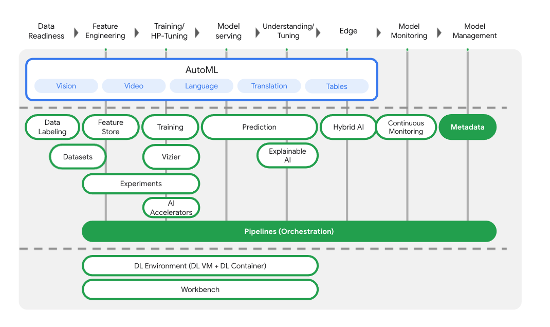
This lab focuses on Vertex Pipelines and Vertex ML Metadata.

If you have any Vertex AI feedback, please see the support page.

Why are ML pipelines useful?

Before we dive in, let's first understand why you would want to use a pipeline. Imagine you're building out an ML workflow that includes processing data, training a model, hyperparameter tuning, evaluation, and model deployment. Each of these steps may have different dependencies, which may become unwieldy if you treat the entire workflow as a monolith. As you begin to scale your ML process, you might want to share your ML workflow with others on your team so they can run it and contribute code. Without a reliable, reproducible process, this can become difficult. With pipelines, each step in your ML process is its own container. This lets you develop steps independently and track the input and output from each step in a reproducible way. You can also schedule or trigger runs of your pipeline based on other events in your Cloud environment, like kicking off a pipeline run when new training data is available.

The tl;dr: pipelines help you automate and reproduce your ML workflow.

3. Cloud environment setup

You'll need a Google Cloud Platform project with billing enabled to run this codelab. To create a project, follow the instructions here.

Start Cloud Shell

In this lab you're going to work in a Cloud Shell session, which is a command interpreter hosted by a virtual machine running in Google's cloud. You could just as easily run this section locally on your own computer, but using Cloud Shell gives everyone access to a reproducible experience in a consistent environment. After the lab, you're welcome to retry this section on your own computer.

The first time you make a request in Cloud Shell requiring authorization, you will see an "Authorize Cloud Shell" dialog like the one shown below, to which you may safely click the "Authorize" button.

Activate Cloud Shell

From the top right of the Cloud Console, click the button below to Activate Cloud Shell:

If you've never started Cloud Shell before, you're presented with an intermediate screen (below the fold) describing what it is. If that's the case, click Continue (and you won't ever see it again). Here's what that one-time screen looks like:

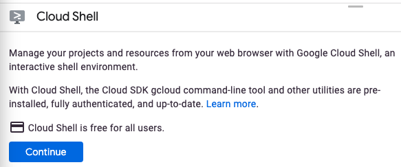
It should only take a few moments to provision and connect to Cloud Shell.

This virtual machine is loaded with all the development tools you need. It offers a persistent 5GB home directory and runs in Google Cloud, greatly enhancing network performance and authentication. Much, if not all, of your work in this codelab can be done with simply a browser or your Chromebook.

Once connected to Cloud Shell, you should see that you are already authenticated and that the project is already set to your project ID.

Run the following command in Cloud Shell to confirm that you are authenticated:

gcloud auth list

Command output

 Credentialed Accounts
ACTIVE  ACCOUNT
*       <my_account>@<my_domain.com>

To set the active account, run:
    $ gcloud config set account `ACCOUNT`

Note: The gcloud command-line tool is the powerful and unified command-line tool in Google Cloud. It comes preinstalled in Cloud Shell. You will notice its support for tab completion. For more information, see gcloud command-line tool overview.

Run the following command in Cloud Shell to confirm that the gcloud command knows about your project:

gcloud config list project

Command output

[core]
project = <PROJECT_ID>

If it is not, you can set it with this command:

gcloud config set project <PROJECT_ID>

Command output

Updated property [core/project].

Cloud Shell has a few environment variables, including GOOGLE_CLOUD_PROJECT which contains the name of our current Cloud project. We'll use this in various places throughout this lab. You can see it by running:

echo $GOOGLE_CLOUD_PROJECT

Enable APIs

In later steps, you'll see where these services are needed (and why), but for now, run this command to give your project access to the Compute Engine, Container Registry, and Vertex AI services:

gcloud services enable compute.googleapis.com         \
                       containerregistry.googleapis.com  \
                       aiplatform.googleapis.com

This should produce a successful message similar to this one:

Operation "operations/acf.cc11852d-40af-47ad-9d59-477a12847c9e" finished successfully.

Create a Cloud Storage Bucket

To run a training job on Vertex AI, we'll need a storage bucket to store our saved model assets. The bucket needs to be regional. We're using us-central here, but you are welcome to use another region (just replace it throughout this lab). If you already have a bucket you can skip this step.

Run the following commands in your Cloud Shell terminal to create a bucket:

BUCKET_NAME=gs://$GOOGLE_CLOUD_PROJECT-bucket
gsutil mb -l us-central1 $BUCKET_NAME

Next we'll give our compute service account access to this bucket. This will ensure that Vertex Pipelines has the necessary permissions to write files to this bucket. Run the following command to add this permission:

gcloud projects describe $GOOGLE_CLOUD_PROJECT > project-info.txt
PROJECT_NUM=$(cat project-info.txt | sed -nre 's:.*projectNumber\: (.*):\1:p')
SVC_ACCOUNT="${PROJECT_NUM//\'/}[e-mail]"
gcloud projects add-iam-policy-binding $GOOGLE_CLOUD_PROJECT --member serviceAccount:$SVC_ACCOUNT --role roles/storage.objectAdmin

Create a Vertex AI Workbench instance

From the Vertex AI section of your Cloud Console, click on Workbench:

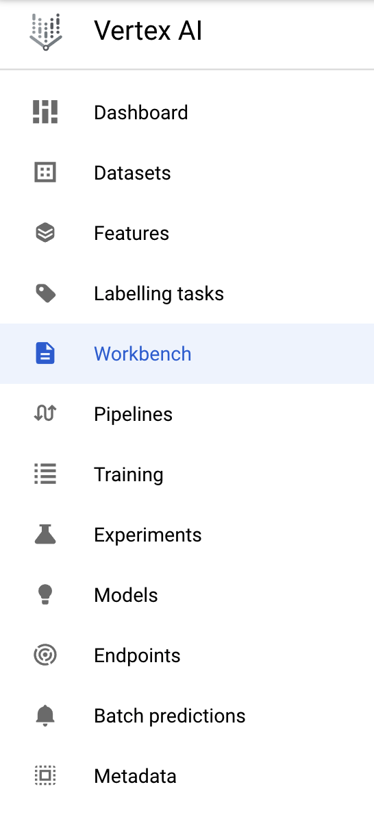
From there, within user-managed notebooks, click New Notebook:

Then select the TensorFlow Enterprise 2.3 (with LTS) instance type without GPUs:

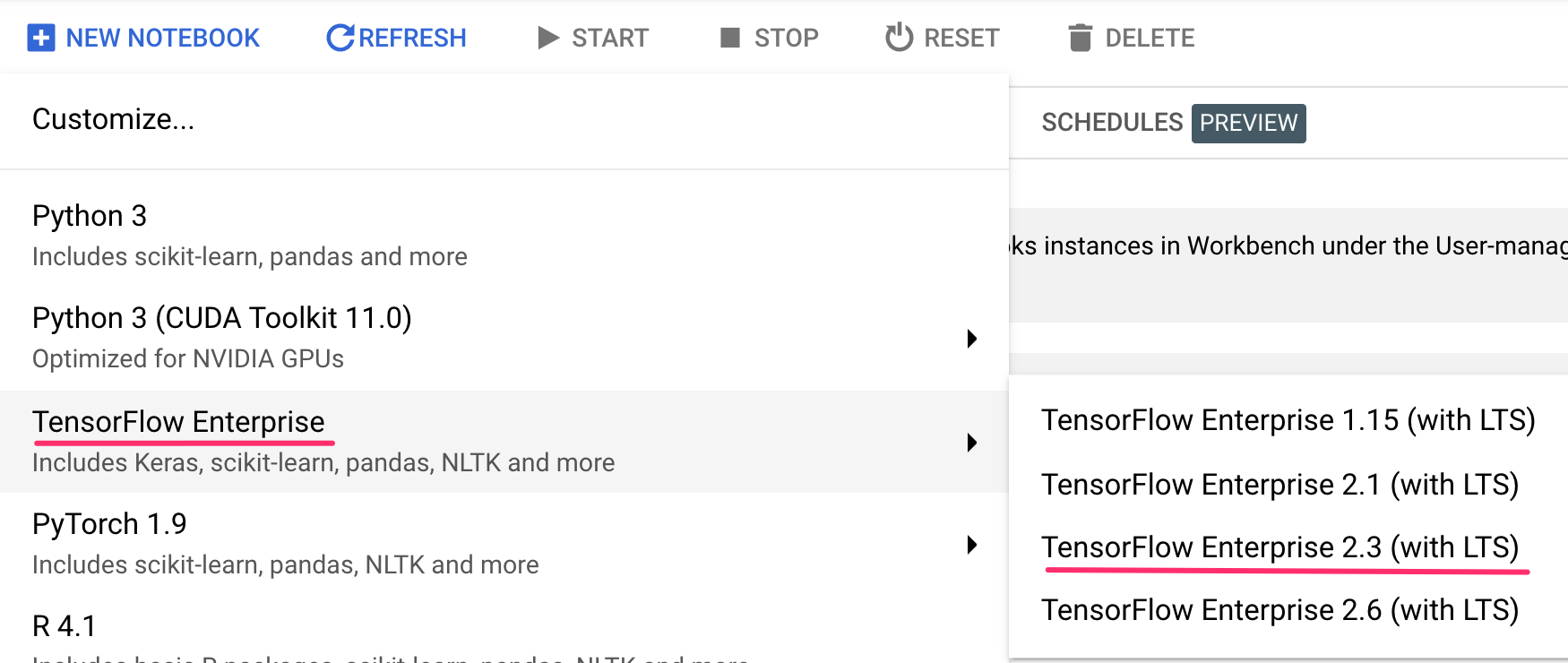
Use the default options and then click Create.

Open your Notebook

Once the instance has been created, select Open JupyterLab:

4. Vertex Pipelines setup

There are a few additional libraries we'll need to install in order to use Vertex Pipelines:

• Kubeflow Pipelines: This is the SDK we'll be using to build our pipeline. Vertex Pipelines supports running pipelines built with both Kubeflow Pipelines or TFX.
• Vertex AI SDK: This SDK optimizes the experience for calling the Vertex AI API. We'll use it to run our pipeline on Vertex AI.

Create Python notebook and install libraries

First, from the Launcher menu in your Notebook instance, create a notebook by selecting Python 3:

You can access the Launcher menu by clicking on the + sign in the top left of your notebook instance.

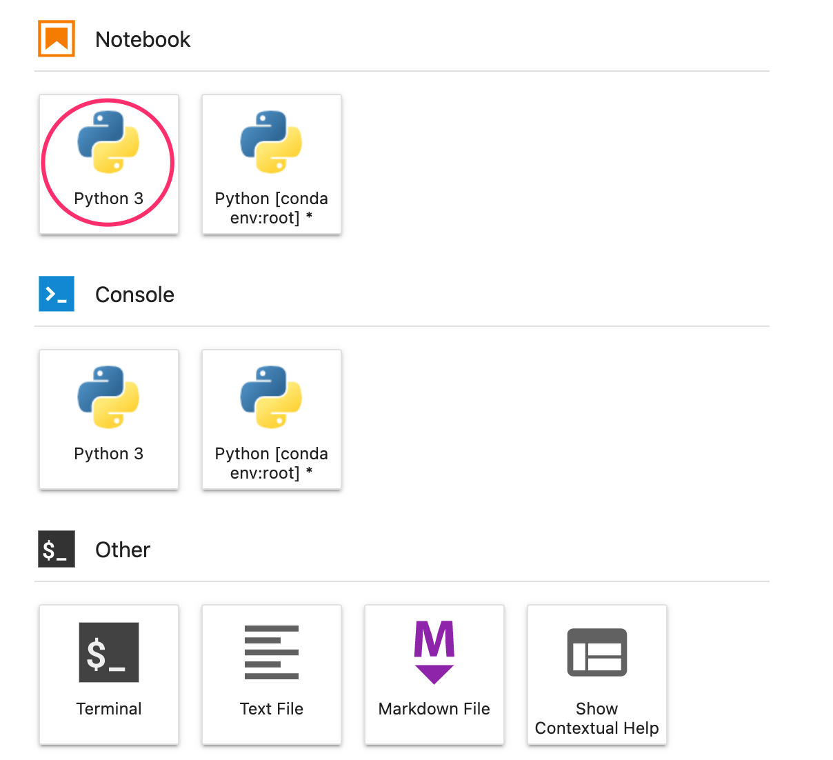
To install both services we'll be using in this lab, first set the user flag in a notebook cell:

USER_FLAG = "--user"

Then run the following from your notebook:

!pip3 install {USER_FLAG} google-cloud-aiplatform==1.7.0
!pip3 install {USER_FLAG} kfp==1.8.9

After installing these packages you'll need to restart the kernel:

import os

if not os.getenv("IS_TESTING"):
    # Automatically restart kernel after installs
    import IPython

    app = IPython.Application.instance()
    app.kernel.do_shutdown(True)

Next, check that you have correctly installed KFP SDK version. It should be >=1.8:

!python3 -c "import kfp; print('KFP SDK version: {}'.format(kfp.__version__))"

Then confirm that your Vertex AI SDK version is >= 1.6.2:

!pip list | grep aiplatform

Set your project ID and bucket

Throughout this lab you'll reference your Cloud project ID and the bucket you created earlier. Next we'll create variables for each of those.

If you don't know your project ID you may be able to get it by running the following:

import os
PROJECT_ID = ""

# Get your Google Cloud project ID from gcloud
if not os.getenv("IS_TESTING"):
    shell_output=!gcloud config list --format 'value(core.project)' 2>/dev/null
    PROJECT_ID = shell_output[0]
    print("Project ID: ", PROJECT_ID)

Otherwise, set it here:

if PROJECT_ID == "" or PROJECT_ID is None:
    PROJECT_ID = "your-project-id"  # @param {type:"string"}

Then create a variable to store your bucket name. If you created it in this lab, the following will work. Otherwise, you'll need to set this manually:

BUCKET_NAME="gs://" + PROJECT_ID + "-bucket"

Import libraries

Add the following to import the libraries we'll be using throughout this codelab:

import matplotlib.pyplot as plt
import pandas as pd

from kfp.v2 import compiler, dsl
from kfp.v2.dsl import pipeline, component, Artifact, Dataset, Input, Metrics, Model, Output, InputPath, OutputPath

from google.cloud import aiplatform

# We'll use this namespace for metadata querying
from google.cloud import aiplatform_v1

Define constants

The last thing we need to do before building our pipeline is define some constant variables. PIPELINE_ROOT is the Cloud Storage path where the artifacts created by our pipeline will be written. We're using us-central1 as the region here, but if you used a different region when you created your bucket, update the REGION variable in the code below:

PATH=%env PATH
%env PATH={PATH}:/home/jupyter/.local/bin
REGION="us-central1"

PIPELINE_ROOT = f"{BUCKET_NAME}/pipeline_root/"
PIPELINE_ROOT

After running the code above, you should see the root directory for your pipeline printed. This is the Cloud Storage location where the artifacts from your pipeline will be written. It will be in the format of gs://YOUR-BUCKET-NAME/pipeline_root/

5. Creating a 3-step pipeline with custom components

The focus of this lab is on understanding metadata from pipeline runs. In order to do that, we'll need a pipeline to run on Vertex Pipelines, which is where we'll start. Here we'll define a 3-step pipeline with the following custom components:

• get_dataframe: Retrieve data from a BigQuery table and convert it into a Pandas DataFrame
• train_sklearn_model: Use the Pandas DataFrame to train and export a Scikit Learn model, along with some metrics
• deploy_model: Deploy the exported Scikit Learn model to an endpoint in Vertex AI

In this pipeline, we'll use the UCI Machine Learning Dry beans dataset, from: KOKLU, M. and OZKAN, I.A., (2020), "Multiclass Classification of Dry Beans Using Computer Vision and Machine Learning Techniques."In Computers and Electronics in Agriculture, 174, 105507. DOI.

This is a tabular dataset, and in our pipeline we'll use the dataset to train, evaluate, and deploy a Scikit-learn model that classifies beans into one of 7 types based on their characteristics. Let's start coding!

Create Python function based components

Using the KFP SDK, we can create components based on Python functions. We'll use that for the 3 components in this pipeline.

Download BigQuery data and convert to CSV

First, we'll build the get_dataframe component:

@component(
    packages_to_install=["google-cloud-bigquery", "pandas", "pyarrow", "db-dtypes"],
    base_image="python:3.9",
    output_component_file="create_dataset.yaml"
)
def get_dataframe(
    bq_table: str,
    output_data_path: OutputPath("Dataset")
):
    from google.cloud import bigquery
    import pandas as pd
    import os

    project_number = os.environ["CLOUD_ML_PROJECT_ID"]
    bqclient = bigquery.Client(project=project_number)
    table = bigquery.TableReference.from_string(
        bq_table
    )
    rows = bqclient.list_rows(
        table
    )
    dataframe = rows.to_dataframe(
        create_bqstorage_client=True,
    )
    dataframe = dataframe.sample(frac=1, random_state=2)
    dataframe.to_csv(output_data_path)

Let's take a closer look at what's happening in this component:

• The @component decorator compiles this function to a component when the pipeline is run. You'll use this anytime you write a custom component.
• The base_image parameter specifies the container image this component will use.
• This component will use a few Python libraries, which we specify via the packages_to_install parameter.
• The output_component_file parameter is optional, and specifies the yaml file to write the compiled component to. After running the cell you should see that file written to your notebook instance. If you wanted to share this component with someone, you could send them the generated yaml file and have them load it with the following:

# This is optional, it shows how to load a component from a yaml file
# dataset_component = kfp.components.load_component_from_file('./create_dataset.yaml')

• Next, this component uses the BigQuery Python client library to download our data from BigQuery into a Pandas DataFrame, and then creates an output artifact of that data as a CSV file. This will be passed as input to our next component

Create a component to train a Scikit-learn model

In this component we'll take the CSV we generated previously and use it to train a Scikit-learn decision tree model. This component exports the resulting Scikit model, along with a Metrics artifact that includes our model's accuracy, framework, and size of the dataset used to train it:

@component(
    packages_to_install=["sklearn", "pandas", "joblib", "db-dtypes"],
    base_image="python:3.9",
    output_component_file="beans_model_component.yaml",
)
def sklearn_train(
    dataset: Input[Dataset],
    metrics: Output[Metrics],
    model: Output[Model]
):
    from sklearn.tree import DecisionTreeClassifier
    from sklearn.metrics import roc_curve
    from sklearn.model_selection import train_test_split
    from joblib import dump

    import pandas as pd
    df = pd.read_csv(dataset.path)
    labels = df.pop("Class").tolist()
    data = df.values.tolist()
    x_train, x_test, y_train, y_test = train_test_split(data, labels)

    skmodel = DecisionTreeClassifier()
    skmodel.fit(x_train,y_train)
    score = skmodel.score(x_test,y_test)
    print('accuracy is:',score)

    metrics.log_metric("accuracy",(score * 100.0))
    metrics.log_metric("framework", "Scikit Learn")
    metrics.log_metric("dataset_size", len(df))
    dump(skmodel, model.path + ".joblib")

Define a component to upload and deploy the model to Vertex AI

Finally, our last component will take the trained model from the previous step, upload it to Vertex AI, and deploy it to an endpoint:

@component(
    packages_to_install=["google-cloud-aiplatform"],
    base_image="python:3.9",
    output_component_file="beans_deploy_component.yaml",
)
def deploy_model(
    model: Input[Model],
    project: str,
    region: str,
    vertex_endpoint: Output[Artifact],
    vertex_model: Output[Model]
):
    from google.cloud import aiplatform

    aiplatform.init(project=project, location=region)

    deployed_model = aiplatform.Model.upload(
        display_name="beans-model-pipeline",
        artifact_uri = model.uri.replace("model", ""),
        serving_container_image_uri="us-docker.pkg.dev/vertex-ai/prediction/sklearn-cpu.0-24:latest"
    )
    endpoint = deployed_model.deploy(machine_type="n1-standard-4")

    # Save data to the output params
    vertex_endpoint.uri = endpoint.resource_name
    vertex_model.uri = deployed_model.resource_name

Here we're using the Vertex AI SDK to upload the model using a pre-built container for prediction. It then deploys the model to an endpoint and returns the URIs to both the model and endpoint resources. Later in this codelab you'll learn more about what it means to return this data as artifacts.

Define and compile the pipeline

Now that we've defined our three components, next we'll create our pipeline definition. This describes how input and output artifacts flow between steps:

@pipeline(
    # Default pipeline root. You can override it when submitting the pipeline.
    pipeline_root=PIPELINE_ROOT,
    # A name for the pipeline.
    name="mlmd-pipeline",
)
def pipeline(
    bq_table: str = "",
    output_data_path: str = "data.csv",
    project: str = PROJECT_ID,
    region: str = REGION
):
    dataset_task = get_dataframe(bq_table)

    model_task = sklearn_train(
        dataset_task.output
    )

    deploy_task = deploy_model(
        model=model_task.outputs["model"],
        project=project,
        region=region
    )

The following will generate a JSON file that you'll use to run the pipeline:

compiler.Compiler().compile(
    pipeline_func=pipeline, package_path="mlmd_pipeline.json"
)

Start two pipeline runs

Next we'll kick off two runs of our pipeline. First let's define a timestamp to use for our pipeline job IDs:

from datetime import datetime

TIMESTAMP = datetime.now().strftime("%Y%m%d%H%M%S")

Remember that our pipeline takes one parameter when we run it: the bq_table we want to use for training data. This pipeline run will use a smaller version of the beans dataset:

run1 = aiplatform.PipelineJob(
    display_name="mlmd-pipeline",
    template_path="mlmd_pipeline.json",
    job_id="mlmd-pipeline-small-{0}".format(TIMESTAMP),
    parameter_values={"bq_table": "sara-vertex-demos.beans_demo.small_dataset"},
    enable_caching=True,
)

Next, create another pipeline run using a larger version of the same dataset.

run2 = aiplatform.PipelineJob(
    display_name="mlmd-pipeline",
    template_path="mlmd_pipeline.json",
    job_id="mlmd-pipeline-large-{0}".format(TIMESTAMP),
    parameter_values={"bq_table": "sara-vertex-demos.beans_demo.large_dataset"},
    enable_caching=True,
)

Finally, kick off pipeline executions for both runs. It's best to do this in two separate notebook cells so you can see the output for each run.

run1.submit()

Then, kick off the second run:

run2.submit()

After running this cell, you'll see a link to view each pipeline in the Vertex AI console. Open that link to see more details on your pipeline:

When it completes (this pipeline takes about 10-15 minutes per run), you'll see something like this:

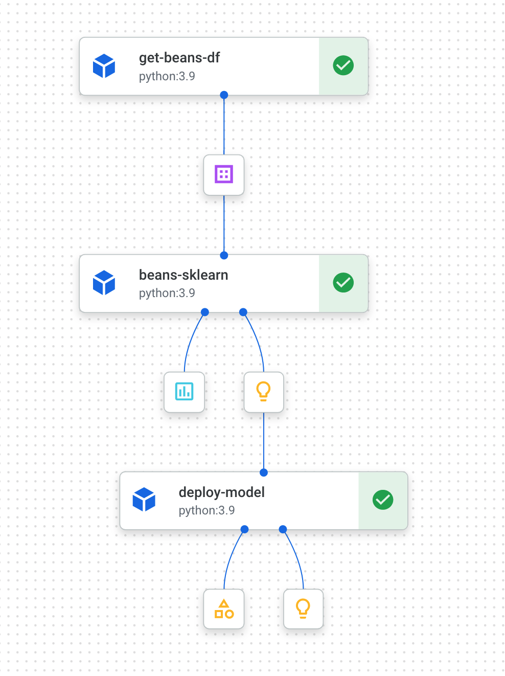
Now that you have two completed pipeline runs, you're ready to take a closer look at pipeline artifacts, metrics, and lineage.

6. Understanding pipeline artifacts and lineage

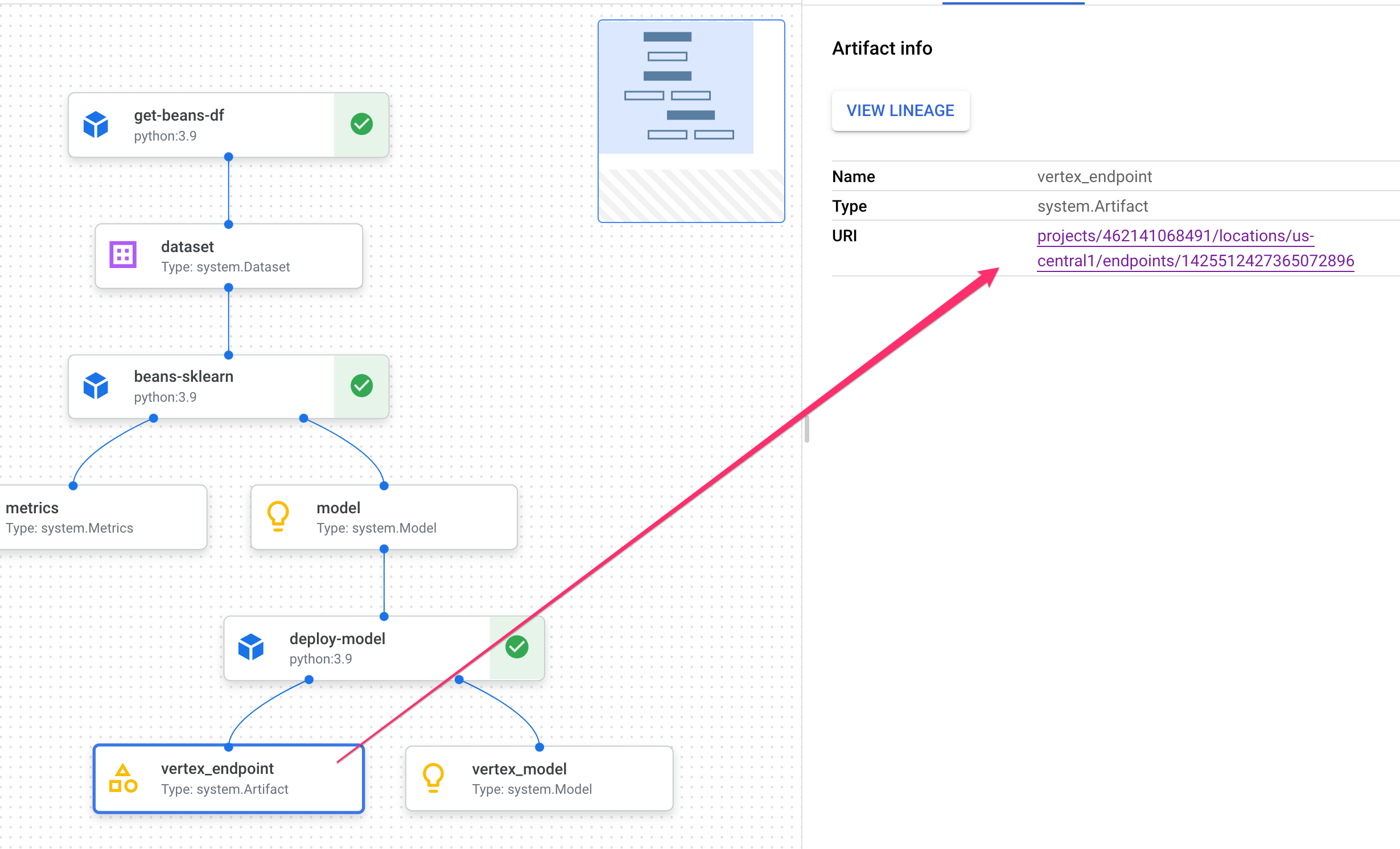
In your pipeline graph, you'll notice small boxes after each step. Those are artifacts, or output generated from a pipeline step. There are many types of artifacts. In this particular pipeline we have dataset, metrics, model, and endpoint artifacts. Click on the Expand Artifacts slider at the top of the UI to see more details on each one:

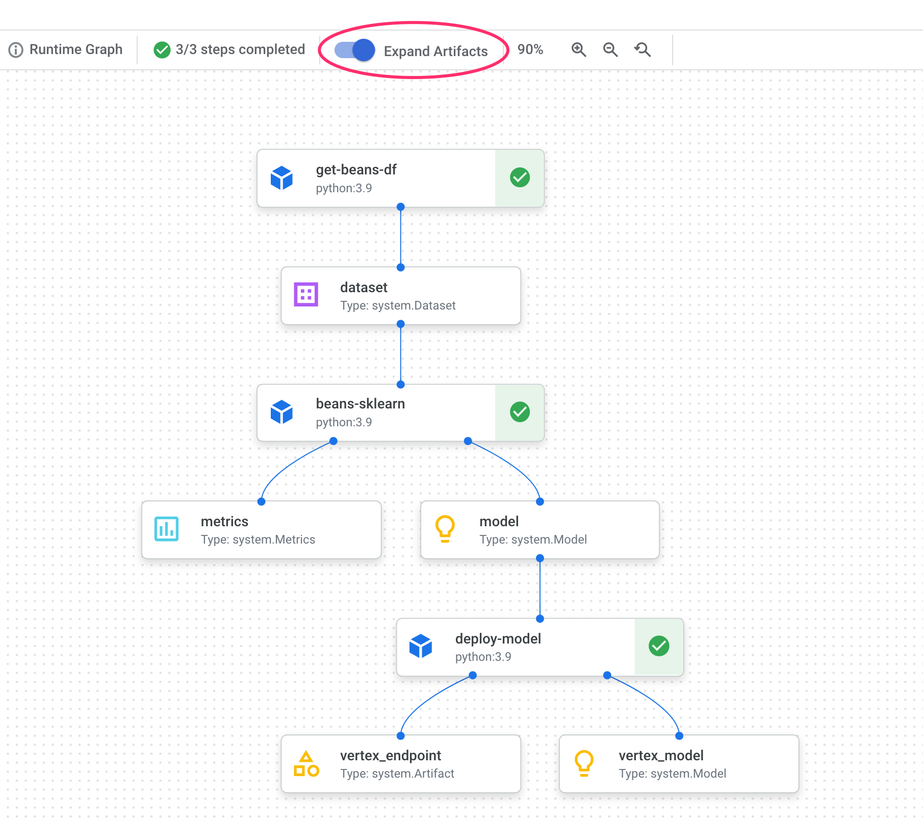
Clicking on an artifact will show you more details on it, including it's URI. For example, clicking on the vertex_endpoint artifact will show you the URI where you can find that deployed endpoint in your Vertex AI console:

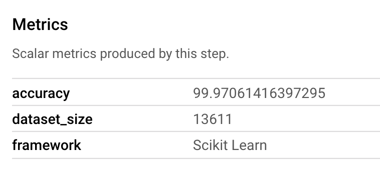
A Metrics artifact lets you pass custom metrics that are associated with a particular pipeline step. In the sklearn_train component of our pipeline, we logged metrics on our model's accuracy, framework, and dataset size. Click on the metrics artifact to see those details:

Every artifact has Lineage, which describes the other artifacts it's connected to. Click on your pipeline's vertex_endpoint artifact again, and then click on the View Lineage button:

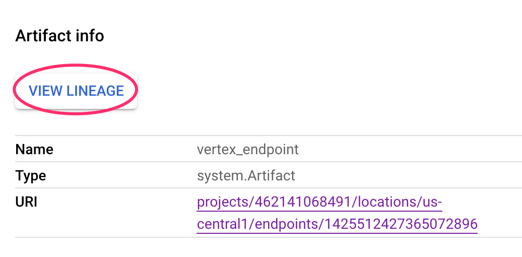
This will open a new tab where you can see all the artifacts connected to the one you've selected. Your lineage graph will look something like this:

This shows us the model, metrics, and dataset associated with this endpoint. Why is this useful? You may have a model deployed to multiple endpoints, or need to know the specific dataset used to train the model deployed to the endpoint you're looking at. The lineage graph helps you understand each artifact in the context of the rest of your ML system. You can also access lineage programmatically, as we'll see later in this codelab.

7. Comparing pipeline runs

Chances are a single pipeline will be run multiple times, maybe with different input parameters, new data, or by people across your team. To keep track of pipeline runs, it would be handy to have a way to compare them according to various metrics. In this section we'll explore two ways to compare runs.

Comparing runs in the Pipelines UI

In the Cloud console, navigate to your Pipelines dashboard. This provides an overview of every pipeline run you've executed. Check the last two runs and then click the Compare button at the top:

This takes us to a page where we can compare input parameters and metrics for each of the runs we've selected. For these two runs, notice the different BigQuery tables, dataset sizes, and accuracy values:

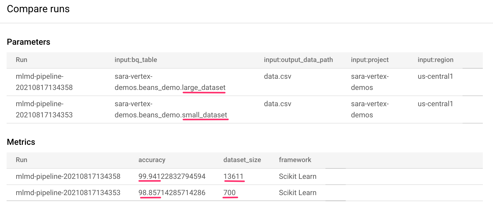
You can use this UI functionality to compare more than two runs, and even runs from different pipelines.

Comparing runs with the Vertex AI SDK

With many pipeline executions, you may want a way to get these comparison metrics programmatically to dig deeper into metrics details and create visualizations.

You can use the aiplatform.get_pipeline_df() method to access run metadata. Here, we'll get metadata for the last two runs of the same pipeline and load it into a Pandas DataFrame. The pipeline parameter here refers to the name we gave our pipeline in our pipeline definition:

df = aiplatform.get_pipeline_df(pipeline="mlmd-pipeline")
df

When you print the DataFrame, you'll see something like this:

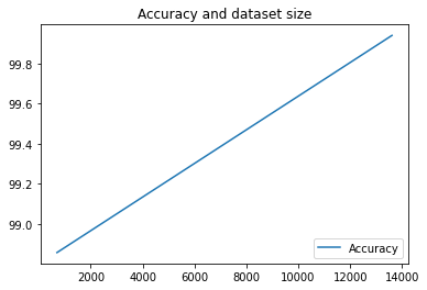
We've only executed our pipeline twice here, but you can imagine how many metrics you'd have with more executions. Next, we'll create a custom visualization with matplotlib to see the relationship between our model's accuracy and the amount of data used for training.

Run the following in a new notebook cell:

plt.plot(df["metric.dataset_size"], df["metric.accuracy"],label="Accuracy")
plt.title("Accuracy and dataset size")
plt.legend(loc=4)
plt.show()

You should see something like this:

8. Querying pipeline metrics

In addition to getting a DataFrame of all pipeline metrics, you may want to programmatically query artifacts created in your ML system. From there you could create a custom dashboard or let others in your organizaiton get details on specific artifacts.

Getting all Model artifacts

To query artifacts in this way, we'll create a MetadataServiceClient:

API_ENDPOINT = "{}-aiplatform.googleapis.com".format(REGION)
metadata_client = aiplatform_v1.MetadataServiceClient(
  client_options={
      "api_endpoint": API_ENDPOINT
  }
)

Next, we'll make a list_artifacts request to that endpoint and pass a filter indicating which artifacts we'd like in our response. First, let's get all the artifacts in our project that are models. To do that, run the following in your notebook:

MODEL_FILTER="schema_title = \"system.Model\""
artifact_request = aiplatform_v1.ListArtifactsRequest(
    parent="projects/{0}/locations/{1}/metadataStores/default".format(PROJECT_ID, REGION),
    filter=MODEL_FILTER
)
model_artifacts = metadata_client.list_artifacts(artifact_request)

The resulting model_artifacts response contains an iterable object for each model artifact in your project, along with associated metadata for each model.

Filtering objects and displaying in a DataFrame

It would be handy if we could more easily visualize the resulting artifact query. Next, let's get all artifacts created after August 10, 2021 with a LIVE state. After we run this request, we'll display the results in a Pandas DataFrame. First, execute the request:

LIVE_FILTER = "create_time > \"2021-08-10T00:00:00-00:00\" AND state = LIVE"
artifact_req = {
    "parent": "projects/{0}/locations/{1}/metadataStores/default".format(PROJECT_ID, REGION),
    "filter": LIVE_FILTER
}
live_artifacts = metadata_client.list_artifacts(artifact_req)

Then, display the results in a DataFrame:

data = {'uri': [], 'createTime': [], 'type': []}

for i in live_artifacts:
    data['uri'].append(i.uri)
    data['createTime'].append(i.create_time)
    data['type'].append(i.schema_title)

df = pd.DataFrame.from_dict(data)
df

You'll see something like this:

You can also filter artifacts based on other criteria in addition to what you tried here.

With that, you've finished the lab!

🎉 Congratulations! 🎉

You've learned how to use Vertex AI to:

• Use the Kubeflow Pipelines SDK to build an ML pipeline that creates a dataset in Vertex AI, and trains and deploys a custom Scikit-learn model on that dataset
• Write custom pipeline components that generate artifacts and metadata
• Compare Vertex Pipelines runs, both in the Cloud console and programmatically
• Trace the lineage for pipeline-generated artifacts
• Query your pipeline run metadata

To learn more about different parts of Vertex, check out the documentation.

9. Cleanup

So that you're not charged, it is recommended that you delete the resources created throughout this lab.

Stop or delete your Notebooks instance

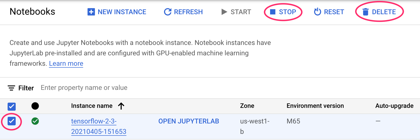
If you'd like to continue using the notebook you created in this lab, it is recommended that you turn it off when not in use. From the Notebooks UI in your Cloud Console, select the notebook and then select Stop. If you'd like to delete the instance entirely, select Delete:

Delete your Vertex AI endpoints

To delete the endpoint you deployed, navigate to the Endpoints section of your Vertex AI console and click the delete icon:

Delete your Cloud Storage bucket

To delete the Storage Bucket, using the Navigation menu in your Cloud Console, browse to Storage, select your bucket, and click Delete: