Utiliser Vertex ML Metadata avec des pipelines

1. Présentation

Dans cet atelier, vous allez apprendre à analyser les métadonnées de vos exécutions Vertex Pipelines avec Vertex ML Metadata.

Objectifs

Vous allez apprendre à effectuer les opérations suivantes :

• Utiliser le SDK Kubeflow Pipelines pour créer un pipeline de ML qui crée un ensemble de données dans Vertex AI, puis entraîne et déploie un modèle Scikit-learn personnalisé sur cet ensemble de données
• Écrire des composants de pipeline personnalisés qui génèrent des artefacts et des métadonnées.
• Comparer les exécutions de Vertex Pipelines, dans la console Cloud et par programmation.
• Assurer la traçabilité des artefacts générés par le pipeline
• Interroger les métadonnées d'exécution du pipeline.

Le coût total d'exécution de cet atelier sur Google Cloud est d'environ 2 $.

2. Présentation de Vertex AI

Cet atelier utilise la toute dernière offre de produits d'IA de Google Cloud. Vertex AI simplifie l'expérience de développement en intégrant toutes les offres de ML de Google Cloud. Auparavant, les modèles entraînés avec AutoML et les modèles personnalisés étaient accessibles depuis des services distincts. La nouvelle offre regroupe ces deux types de modèles mais aussi d'autres nouveaux produits en une seule API. Vous pouvez également migrer des projets existants vers Vertex AI.

Outre les services d'entraînement et de déploiement de modèles, Vertex AI inclut également divers produits MLOps comme Vertex Pipelines, ML Metadata, Model Monitoring, Feature Store, etc. Toutes les offres de produits de Vertex AI sont répertoriées dans le schéma ci-dessous.

Cet atelier porte sur Vertex Pipelines et Vertex ML Metadata.

Pour envoyer un commentaire sur Vertex AI, veuillez consulter la page d'assistance.

Pourquoi utiliser des pipelines de ML ?

Avant d'entrer dans le vif du sujet, vous devez comprendre les avantages d'un pipeline. Imaginez que vous créez un workflow de ML incluant le traitement de données, l'entraînement d'un modèle, le réglage d'hyperparamètres, l'évaluation et le déploiement d'un modèle. Chacune de ces étapes peut avoir des dépendances différentes, ce qui peut se révéler problématique si vous traitez l'ensemble du workflow comme un monolithe. Lorsque vous commencerez le scaling de votre processus de ML, vous souhaiterez peut-être partager votre workflow de ML avec le reste de votre équipe, afin qu'elle puisse l'exécuter et participer à l'écriture du code. Cela peut s'avérer difficile sans un processus fiable et reproductible. Avec les pipelines, chaque étape de votre processus de ML est son propre conteneur. Ainsi, vous pouvez développer des étapes de façon indépendante et suivre les entrées et sorties de chaque étape de manière reproductible. Vous pouvez également planifier ou déclencher des exécutions de votre pipeline en fonction d'autres événements dans votre environnement cloud. Par exemple, vous pouvez exécuter un pipeline lorsque de nouvelles données d'entraînement sont disponibles.

En résumé : les pipelines vous aident à automatiser et à reproduire votre workflow de ML.

3. Configurer l'environnement cloud

Pour suivre cet atelier de programmation, vous aurez besoin d'un projet Google Cloud Platform dans lequel la facturation est activée. Pour créer un projet, suivez ces instructions.

Démarrer Cloud Shell

Dans cet atelier, vous allez travailler dans une session Cloud Shell. Cet environnement est un interpréteur de commandes hébergé sur une machine virtuelle qui s'exécute dans le cloud de Google. Vous pourriez tout aussi facilement effectuer les tâches de cette section en local sur votre propre ordinateur, mais le fait d'utiliser Cloud Shell permet à chacun de bénéficier d'une expérience reproductible dans un environnement cohérent. Après l'atelier, libre à vous de reproduire cette section sur votre ordinateur.

Étant donné que la première requête que vous enverrez dans Cloud Shell nécessite une autorisation, vous verrez une boîte de dialogue "Autorisez Cloud Shell" comme celle ci-dessous. Vous pouvez cliquer sur le bouton "Autoriser" sans problème.

Activer Cloud Shell

En haut à droite de la console Cloud, cliquez sur le bouton Activer Cloud Shell :

Si vous n'avez jamais démarré Cloud Shell auparavant, un écran intermédiaire s'affiche en dessous de la ligne de flottaison, décrivant de quoi il s'agit. Si tel est le cas, cliquez sur Continuer. Cet écran ne s'affiche qu'une seule fois. Voici à quoi il ressemble :

Le provisionnement et la connexion à Cloud Shell ne devraient pas prendre plus de quelques minutes.

Cette machine virtuelle contient tous les outils de développement dont vous avez besoin. Elle comprend un répertoire d'accueil persistant de 5 Go et s'exécute sur Google Cloud, ce qui améliore nettement les performances du réseau et l'authentification. Vous pouvez réaliser une grande partie, voire la totalité, des activités de cet atelier dans un simple navigateur ou sur votre Chromebook.

Une fois connecté à Cloud Shell, vous êtes en principe authentifié et le projet est défini avec votre ID de projet.

Exécutez la commande suivante dans Cloud Shell pour vérifier que vous êtes authentifié :

gcloud auth list

Résultat de la commande

 Credentialed Accounts
ACTIVE  ACCOUNT
*       <my_account>@<my_domain.com>

To set the active account, run:
    $ gcloud config set account `ACCOUNT`

Remarque : gcloud est l'outil de ligne de commande performant et unifié de Google Cloud. Il est préinstallé dans Cloud Shell. Il est également compatible avec la saisie semi-automatique via la touche de tabulation. Pour en savoir plus, consultez la section de présentation de l'outil de ligne de commande gcloud.

Exécutez la commande suivante dans Cloud Shell pour vérifier que la commande gcloud connaît votre projet :

gcloud config list project

Résultat de la commande

[core]
project = <PROJECT_ID>

Si vous obtenez un résultat différent, exécutez cette commande :

gcloud config set project <PROJECT_ID>

Résultat de la commande

Updated property [core/project].

Cloud Shell comporte quelques variables d'environnement, dont GOOGLE_CLOUD_PROJECT, qui contient le nom de notre projet Cloud actuel. Nous l'utiliserons à plusieurs endroits tout au long de cet atelier. Pour la voir, exécutez la commande suivante :

echo $GOOGLE_CLOUD_PROJECT

Activer les API

Dans les étapes suivantes, vous verrez où ces services sont requis (et pourquoi). Mais pour l'instant, exécutez la commande ci-dessous pour autoriser votre projet à accéder aux services Compute Engine, Container Registry et Vertex AI :

gcloud services enable compute.googleapis.com         \
                       containerregistry.googleapis.com  \
                       aiplatform.googleapis.com

Un message semblable à celui qui suit s'affiche pour vous indiquer que l'opération s'est correctement déroulée :

Operation "operations/acf.cc11852d-40af-47ad-9d59-477a12847c9e" finished successfully.

Créer un bucket Cloud Storage

Pour exécuter un job d'entraînement sur Vertex AI, nous avons besoin d'un bucket de stockage dans lequel enregistrer les ressources de modèle. Ce bucket doit être régional. Nous utilisons ici us-central, mais vous pouvez utiliser une autre région (il vous suffit d'effectuer le remplacement tout au long de cet atelier). Si vous disposez déjà d'un bucket, vous pouvez ignorer cette étape.

Exécutez les commandes suivantes dans votre terminal Cloud Shell afin de créer un bucket :

BUCKET_NAME=gs://$GOOGLE_CLOUD_PROJECT-bucket
gsutil mb -l us-central1 $BUCKET_NAME

Nous allons ensuite autoriser notre compte de service Compute à accéder à ce bucket. Ainsi, Vertex Pipelines disposera des autorisations nécessaires pour écrire des fichiers dans ce bucket. Exécutez la commande suivante pour ajouter cette autorisation :

gcloud projects describe $GOOGLE_CLOUD_PROJECT > project-info.txt
PROJECT_NUM=$(cat project-info.txt | sed -nre 's:.*projectNumber\: (.*):\1:p')
SVC_ACCOUNT="${PROJECT_NUM//\'/}[e-mail]"
gcloud projects add-iam-policy-binding $GOOGLE_CLOUD_PROJECT --member serviceAccount:$SVC_ACCOUNT --role roles/storage.objectAdmin

Créer une instance Vertex AI Workbench

Dans la section Vertex AI de Cloud Console, cliquez sur Workbench :

Dans Notebooks gérés par l'utilisateur, cliquez sur Nouveau notebook :

Sélectionnez ensuite le type d'instance TensorFlow Enterprise 2.3 (avec LTS) sans GPU :

Utilisez les options par défaut, puis cliquez sur Créer.

Ouvrir votre notebook

Une fois l'instance créée, sélectionnez Ouvrir JupyterLab :

4. Configuration de Vertex Pipelines

Pour utiliser Vertex Pipelines, il est nécessaire d'installer quelques bibliothèques supplémentaires.

• Kubeflow Pipelines : le SDK que nous utiliserons pour créer notre pipeline. Vertex Pipelines est compatible avec l'exécution de pipelines créés avec Kubeflow Pipelines ou TFX.
• SDK Vertex AI : ce SDK optimise l'expérience d'appel de l'API Vertex AI. Nous l'utiliserons pour exécuter notre pipeline sur Vertex AI.

Créer un notebook Python et installer les bibliothèques

Tout d'abord, dans le menu de lancement de votre instance de notebook, créez un notebook en sélectionnant Python 3 :

Pour accéder au menu de lancement, cliquez sur le signe + en haut à gauche de votre instance de notebook.

Pour installer les deux services que nous utiliserons dans cet atelier, vous devez d'abord définir l'option utilisateur dans une cellule du notebook :

USER_FLAG = "--user"

Exécutez ensuite les commandes suivantes depuis votre notebook :

!pip3 install {USER_FLAG} google-cloud-aiplatform==1.7.0
!pip3 install {USER_FLAG} kfp==1.8.9

Une fois ces packages installés, vous devrez redémarrer le kernel :

import os

if not os.getenv("IS_TESTING"):
    # Automatically restart kernel after installs
    import IPython

    app = IPython.Application.instance()
    app.kernel.do_shutdown(True)

Ensuite, vérifiez que vous avez correctement installé la version du SDK KFP. Elle doit être supérieure ou égale à 1,8 :

!python3 -c "import kfp; print('KFP SDK version: {}'.format(kfp.__version__))"

Ensuite, vérifiez que votre version du SDK Vertex AI est >= 1.6.2 :

!pip list | grep aiplatform

Définir l'ID de votre projet et votre bucket

Au cours de cet atelier, vous allez référencer votre ID de projet Cloud et le bucket que vous avez créé un peu plus tôt. Nous allons à présent créer des variables pour chacun d'eux.

Si vous ne connaissez pas votre ID de projet, vous pouvez l'obtenir en exécutant la commande suivante :

import os
PROJECT_ID = ""

# Get your Google Cloud project ID from gcloud
if not os.getenv("IS_TESTING"):
    shell_output=!gcloud config list --format 'value(core.project)' 2>/dev/null
    PROJECT_ID = shell_output[0]
    print("Project ID: ", PROJECT_ID)

Sinon, définissez-le ici :

if PROJECT_ID == "" or PROJECT_ID is None:
    PROJECT_ID = "your-project-id"  # @param {type:"string"}

Ensuite, créez une variable pour stocker le nom de votre bucket. Si vous l'avez créée au cours de cet atelier, les étapes suivantes devraient fonctionner. Sinon, vous devrez la définir manuellement :

BUCKET_NAME="gs://" + PROJECT_ID + "-bucket"

Importer des bibliothèques

Ajoutez le code suivant pour importer les bibliothèques que nous utiliserons dans cet atelier de programmation :

import matplotlib.pyplot as plt
import pandas as pd

from kfp.v2 import compiler, dsl
from kfp.v2.dsl import pipeline, component, Artifact, Dataset, Input, Metrics, Model, Output, InputPath, OutputPath

from google.cloud import aiplatform

# We'll use this namespace for metadata querying
from google.cloud import aiplatform_v1

Définir des constantes

La dernière chose que nous devons faire avant de pouvoir créer notre pipeline est de définir des variables constantes. PIPELINE_ROOT est le chemin d'accès Cloud Storage dans lequel les artefacts créés par notre pipeline seront écrits. Ici, nous utilisons us-central1 comme région, mais si vous avez choisi une autre région lorsque vous avez créé votre bucket, modifiez la variable REGION dans le code ci-dessous :

PATH=%env PATH
%env PATH={PATH}:/home/jupyter/.local/bin
REGION="us-central1"

PIPELINE_ROOT = f"{BUCKET_NAME}/pipeline_root/"
PIPELINE_ROOT

Une fois le code ci-dessus exécuté, le répertoire racine de votre pipeline doit s'afficher. Il s'agit de l'emplacement Cloud Storage dans lequel les artefacts de votre pipeline seront écrits. Elle se présentera au format gs://YOUR-BUCKET-NAME/pipeline_root/.

5. Créer un pipeline en trois étapes avec des composants personnalisés

Cet atelier vise à vous aider à comprendre les métadonnées des exécutions de pipeline. Pour ce faire, nous avons besoin d'un pipeline à exécuter sur Vertex Pipelines. C'est par là que nous allons commencer. Nous allons définir un pipeline en trois étapes avec les composants personnalisés suivants :

• get_dataframe : récupérer les données d'une table BigQuery et les convertir en DataFrame Pandas
• train_sklearn_model : utilisez le DataFrame Pandas pour entraîner et exporter un modèle Scikit-learn, ainsi que certaines métriques.
• deploy_model : Déployez le modèle Scikit-Learn exporté sur un point de terminaison dans Vertex AI.

Dans ce pipeline, nous utiliserons l'ensemble de données Dry beans dataset (haricots secs) de l'UCI Machine Learning, de KOKLU, M. et OZKAN, I.A., (2020), "Multiclass Classification of Dry Beans Using Computer Vision and Machine Learning Techniques." publié dans "Computers and Electronics in Agriculture", 174, 105507. DOI.

Il s'agit d'un ensemble de données tabulaire, que nous utiliserons dans notre pipeline pour entraîner, évaluer et déployer un modèle Scikit-learn qui répartit des haricots en sept types en fonction de leurs caractéristiques. Commençons à coder !

Créer des composants basés sur des fonctions Python

Le SDK KFP nous permet de créer des composants basés sur des fonctions Python. Nous l'utiliserons pour les trois composants de ce pipeline.

Télécharger des données BigQuery et les convertir au format CSV

Commençons par créer le composant get_dataframe :

@component(
    packages_to_install=["google-cloud-bigquery", "pandas", "pyarrow", "db-dtypes"],
    base_image="python:3.9",
    output_component_file="create_dataset.yaml"
)
def get_dataframe(
    bq_table: str,
    output_data_path: OutputPath("Dataset")
):
    from google.cloud import bigquery
    import pandas as pd
    import os

    project_number = os.environ["CLOUD_ML_PROJECT_ID"]
    bqclient = bigquery.Client(project=project_number)
    table = bigquery.TableReference.from_string(
        bq_table
    )
    rows = bqclient.list_rows(
        table
    )
    dataframe = rows.to_dataframe(
        create_bqstorage_client=True,
    )
    dataframe = dataframe.sample(frac=1, random_state=2)
    dataframe.to_csv(output_data_path)

Examinons de plus près ce qui se passe dans ce composant :

• Le décorateur @component compile cette fonction en un composant lorsque le pipeline est exécuté. Vous l'utiliserez à chaque fois que vous écrirez un composant personnalisé.
• Le paramètre base_image spécifie l'image de conteneur que ce composant utilisera.
• Ce composant utilisera quelques bibliothèques Python, que nous spécifions à l'aide du paramètre packages_to_install.
• Le paramètre facultatif output_component_file spécifie le fichier yaml dans lequel écrire le composant compilé. Une fois la cellule exécutée, ce fichier doit être écrit dans votre instance de notebook. Si vous souhaitez partager ce composant avec une autre personne, vous pouvez lui envoyer le fichier yaml qui a été généré afin qu'elle le charge à l'aide de la commande suivante :

# This is optional, it shows how to load a component from a yaml file
# dataset_component = kfp.components.load_component_from_file('./create_dataset.yaml')

• Ensuite, ce composant utilise la bibliothèque cliente Python de BigQuery pour télécharger nos données depuis BigQuery dans un DataFrame Pandas, puis crée un artefact de sortie de ces données sous forme de fichier CSV. Il sera transmis en entrée à notre prochain composant.

Créer un composant pour entraîner un modèle Scikit-learn

Dans ce composant, nous allons prendre le fichier CSV que nous avons généré précédemment et l'utiliser pour entraîner un modèle d'arbre de décision Scikit-learn. Ce composant exporte le modèle Scikit obtenu, ainsi qu'un artefact Metrics qui inclut la précision, le framework et la taille de l'ensemble de données utilisé pour entraîner notre modèle :

@component(
    packages_to_install=["sklearn", "pandas", "joblib", "db-dtypes"],
    base_image="python:3.9",
    output_component_file="beans_model_component.yaml",
)
def sklearn_train(
    dataset: Input[Dataset],
    metrics: Output[Metrics],
    model: Output[Model]
):
    from sklearn.tree import DecisionTreeClassifier
    from sklearn.metrics import roc_curve
    from sklearn.model_selection import train_test_split
    from joblib import dump

    import pandas as pd
    df = pd.read_csv(dataset.path)
    labels = df.pop("Class").tolist()
    data = df.values.tolist()
    x_train, x_test, y_train, y_test = train_test_split(data, labels)

    skmodel = DecisionTreeClassifier()
    skmodel.fit(x_train,y_train)
    score = skmodel.score(x_test,y_test)
    print('accuracy is:',score)

    metrics.log_metric("accuracy",(score * 100.0))
    metrics.log_metric("framework", "Scikit Learn")
    metrics.log_metric("dataset_size", len(df))
    dump(skmodel, model.path + ".joblib")

Définir un composant pour importer et déployer le modèle dans Vertex AI

Enfin, notre dernier composant prendra le modèle entraîné de l'étape précédente, l'importera dans Vertex AI et le déploiera sur un point de terminaison :

@component(
    packages_to_install=["google-cloud-aiplatform"],
    base_image="python:3.9",
    output_component_file="beans_deploy_component.yaml",
)
def deploy_model(
    model: Input[Model],
    project: str,
    region: str,
    vertex_endpoint: Output[Artifact],
    vertex_model: Output[Model]
):
    from google.cloud import aiplatform

    aiplatform.init(project=project, location=region)

    deployed_model = aiplatform.Model.upload(
        display_name="beans-model-pipeline",
        artifact_uri = model.uri.replace("model", ""),
        serving_container_image_uri="us-docker.pkg.dev/vertex-ai/prediction/sklearn-cpu.0-24:latest"
    )
    endpoint = deployed_model.deploy(machine_type="n1-standard-4")

    # Save data to the output params
    vertex_endpoint.uri = endpoint.resource_name
    vertex_model.uri = deployed_model.resource_name

Ici, nous utilisons le SDK Vertex AI pour importer le modèle à l'aide d'un conteneur prédéfini pour la prédiction. Il déploie ensuite le modèle sur un point de terminaison et renvoie les URI des ressources de modèle et de point de terminaison. Plus loin dans cet atelier de programmation, vous en apprendrez davantage sur ce que signifie renvoyer ces données en tant qu'artefacts.

Définir et compiler le pipeline

Maintenant que nous avons défini nos trois composants, nous allons créer notre définition de pipeline. Voici comment les artefacts d'entrée et de sortie circulent entre les étapes :

@pipeline(
    # Default pipeline root. You can override it when submitting the pipeline.
    pipeline_root=PIPELINE_ROOT,
    # A name for the pipeline.
    name="mlmd-pipeline",
)
def pipeline(
    bq_table: str = "",
    output_data_path: str = "data.csv",
    project: str = PROJECT_ID,
    region: str = REGION
):
    dataset_task = get_dataframe(bq_table)

    model_task = sklearn_train(
        dataset_task.output
    )

    deploy_task = deploy_model(
        model=model_task.outputs["model"],
        project=project,
        region=region
    )

Le code suivant génère un fichier JSON qui vous permettra d'exécuter le pipeline :

compiler.Compiler().compile(
    pipeline_func=pipeline, package_path="mlmd_pipeline.json"
)

Démarrer deux exécutions de pipeline

Nous allons ensuite lancer deux exécutions de notre pipeline. Commençons par définir un code temporel à utiliser pour les ID de job de pipeline :

from datetime import datetime

TIMESTAMP = datetime.now().strftime("%Y%m%d%H%M%S")

N'oubliez pas que notre pipeline prend un paramètre lors de son exécution : le bq_table que nous voulons utiliser pour les données d'entraînement. Cette exécution de pipeline utilisera une version plus petite de l'ensemble de données sur les haricots :

run1 = aiplatform.PipelineJob(
    display_name="mlmd-pipeline",
    template_path="mlmd_pipeline.json",
    job_id="mlmd-pipeline-small-{0}".format(TIMESTAMP),
    parameter_values={"bq_table": "sara-vertex-demos.beans_demo.small_dataset"},
    enable_caching=True,
)

Créez ensuite une autre exécution de pipeline à l'aide d'une version plus grande du même ensemble de données.

run2 = aiplatform.PipelineJob(
    display_name="mlmd-pipeline",
    template_path="mlmd_pipeline.json",
    job_id="mlmd-pipeline-large-{0}".format(TIMESTAMP),
    parameter_values={"bq_table": "sara-vertex-demos.beans_demo.large_dataset"},
    enable_caching=True,
)

Enfin, lancez les exécutions de pipeline pour les deux exécutions. Il est préférable de le faire dans deux cellules de notebook distinctes afin de pouvoir voir le résultat de chaque exécution.

run1.submit()

Lancez ensuite la deuxième exécution :

run2.submit()

Après avoir exécuté cette cellule, vous verrez un lien permettant d'afficher chaque pipeline dans la console Vertex AI. Ouvrez ce lien pour en savoir plus sur votre pipeline :

Une fois l'exécution terminée (ce pipeline prend environ 10 à 15 minutes par exécution), vous verrez quelque chose comme ceci :

Maintenant que vous avez deux exécutions de pipeline terminées, vous pouvez examiner de plus près les artefacts, les métriques et la provenance du pipeline.

6. Comprendre les artefacts et la traçabilité des pipelines

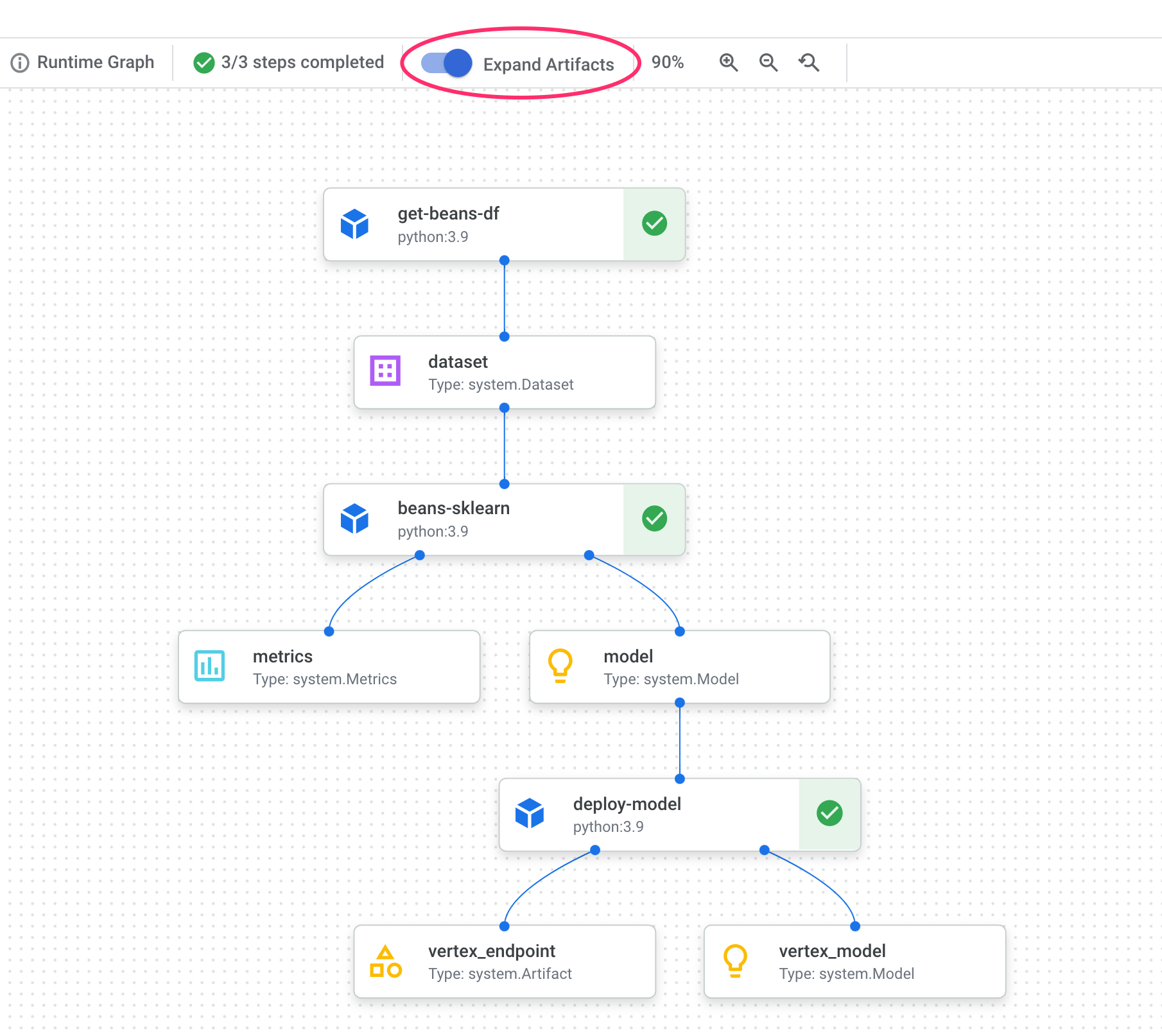
Dans le graphique de votre pipeline, vous remarquerez de petites cases après chaque étape. Il s'agit d'artefacts, ou de résultats générés à partir d'une étape du pipeline. Il existe de nombreux types d'artefacts. Dans ce pipeline particulier, nous avons des artefacts d'ensemble de données, de métriques, de modèle et de point de terminaison. Cliquez sur le curseur Développer les artefacts en haut de l'interface utilisateur pour afficher plus de détails sur chacun d'eux :

En cliquant sur un artefact, vous obtiendrez plus d'informations à son sujet, y compris son URI. Par exemple, si vous cliquez sur l'artefact vertex_endpoint, l'URI du point de terminaison déployé s'affiche dans la console Vertex AI :

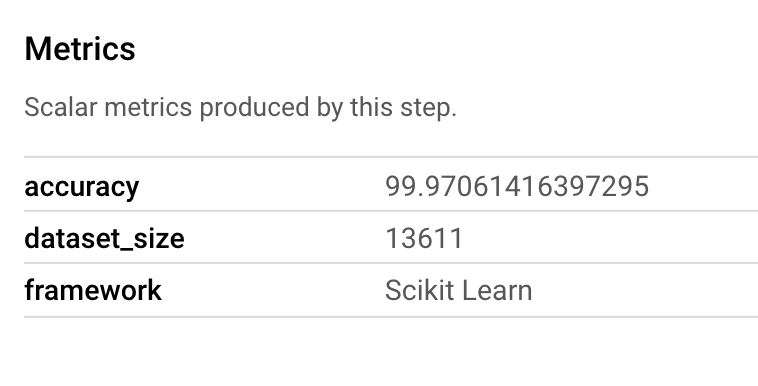
Un artefact Metrics vous permet de transmettre des métriques personnalisées associées à une étape de pipeline spécifique. Dans le composant sklearn_train de notre pipeline, nous avons enregistré des métriques sur la précision, le framework et la taille de l'ensemble de données de notre modèle. Cliquez sur l'artefact de métriques pour afficher ces détails :

Chaque artefact possède une traçabilité qui décrit les autres artefacts auxquels il est connecté. Cliquez à nouveau sur l'artefact vertex_endpoint de votre pipeline, puis sur le bouton Afficher la traçabilité :

Un nouvel onglet s'ouvre, dans lequel vous pouvez voir tous les artefacts associés à celui que vous avez sélectionné. Votre graphique de lignée ressemblera à ceci :

Cela nous montre le modèle, les métriques et l'ensemble de données associés à ce point de terminaison. En quoi est-ce utile ? Il est possible que vous ayez déployé un modèle sur plusieurs points de terminaison ou que vous ayez besoin de connaître l'ensemble de données spécifique utilisé pour entraîner le modèle déployé sur le point de terminaison que vous consultez. Le graphique de traçabilité vous aide à comprendre chaque artefact dans le contexte du reste de votre système de ML. Vous pouvez également accéder à la lignée de manière programmatique, comme nous le verrons plus loin dans cet atelier de programmation.

7. Comparer les exécutions de pipeline

Il est probable qu'un même pipeline soit exécuté plusieurs fois, peut-être avec des paramètres d'entrée différents, de nouvelles données ou par des membres de votre équipe. Pour suivre les exécutions de pipeline, il serait utile de pouvoir les comparer selon différentes métriques. Dans cette section, nous allons explorer deux façons de comparer les exécutions.

Comparer les exécutions dans l'UI Pipelines

Dans la console Cloud, accédez au tableau de bord Pipelines. Vous y trouverez un aperçu de chaque exécution de pipeline que vous avez effectuée. Cochez les deux dernières exécutions, puis cliquez sur le bouton Comparer en haut de la page :

Nous sommes alors redirigés vers une page où nous pouvons comparer les paramètres d'entrée et les métriques de chacune des exécutions que nous avons sélectionnées. Pour ces deux exécutions, notez les différences entre les tables BigQuery, la taille des ensembles de données et les valeurs de précision :

Vous pouvez utiliser cette fonctionnalité d'UI pour comparer plus de deux exécutions, et même des exécutions de différents pipelines.

Comparer des exécutions avec le SDK Vertex AI

Avec de nombreuses exécutions de pipeline, vous pouvez souhaiter obtenir ces métriques de comparaison de manière programmatique pour examiner plus en détail les métriques et créer des visualisations.

La méthode aiplatform.get_pipeline_df() vous permet d'accéder aux métadonnées des exécutions. Voici comment obtenir les métadonnées des deux dernières exécutions du même pipeline et les charger dans un DataFrame Pandas. Le paramètre pipeline fait ici référence au nom que nous avons donné à notre pipeline dans sa définition :

df = aiplatform.get_pipeline_df(pipeline="mlmd-pipeline")
df

Lorsque vous imprimerez le DataFrame, vous verrez quelque chose comme ceci :

Nous n'avons exécuté notre pipeline que deux fois ici, mais vous pouvez imaginer le nombre de métriques que vous auriez avec plus d'exécutions. Ensuite, nous allons créer une visualisation personnalisée avec matplotlib pour voir la relation entre la précision de notre modèle et la quantité de données utilisées pour l'entraînement.

Exécutez le code suivant dans une nouvelle cellule de notebook :

plt.plot(df["metric.dataset_size"], df["metric.accuracy"],label="Accuracy")
plt.title("Accuracy and dataset size")
plt.legend(loc=4)
plt.show()

L'écran qui s'affiche devrait ressembler à ce qui suit :

8. Interroger les métriques du pipeline

En plus d'obtenir un DataFrame de toutes les métriques de pipeline, vous pouvez interroger de manière programmatique les artefacts créés dans votre système de ML. Vous pouvez ensuite créer un tableau de bord personnalisé ou permettre aux autres membres de votre organisation d'obtenir des informations sur des artefacts spécifiques.

Obtenir tous les artefacts de modèle

Pour interroger les artefacts de cette manière, nous allons créer un MetadataServiceClient :

API_ENDPOINT = "{}-aiplatform.googleapis.com".format(REGION)
metadata_client = aiplatform_v1.MetadataServiceClient(
  client_options={
      "api_endpoint": API_ENDPOINT
  }
)

Ensuite, nous allons envoyer une requête list_artifacts à ce point de terminaison et transmettre un filtre indiquant les artefacts que nous souhaitons inclure dans notre réponse. Commençons par récupérer tous les artefacts de notre projet qui sont des modèles. Pour ce faire, exécutez la commande suivante dans votre notebook :

MODEL_FILTER="schema_title = \"system.Model\""
artifact_request = aiplatform_v1.ListArtifactsRequest(
    parent="projects/{0}/locations/{1}/metadataStores/default".format(PROJECT_ID, REGION),
    filter=MODEL_FILTER
)
model_artifacts = metadata_client.list_artifacts(artifact_request)

La réponse model_artifacts obtenue contient un objet itérable pour chaque artefact de modèle de votre projet, ainsi que les métadonnées associées pour chaque modèle.

Filtrer des objets et les afficher dans un DataFrame

Il serait utile de pouvoir visualiser plus facilement la requête d'artefact résultante. Ensuite, récupérons tous les artefacts créés après le 10 août 2021 avec l'état LIVE. Une fois cette requête exécutée, nous afficherons les résultats dans un DataFrame Pandas. Tout d'abord, exécutez la requête :

LIVE_FILTER = "create_time > \"2021-08-10T00:00:00-00:00\" AND state = LIVE"
artifact_req = {
    "parent": "projects/{0}/locations/{1}/metadataStores/default".format(PROJECT_ID, REGION),
    "filter": LIVE_FILTER
}
live_artifacts = metadata_client.list_artifacts(artifact_req)

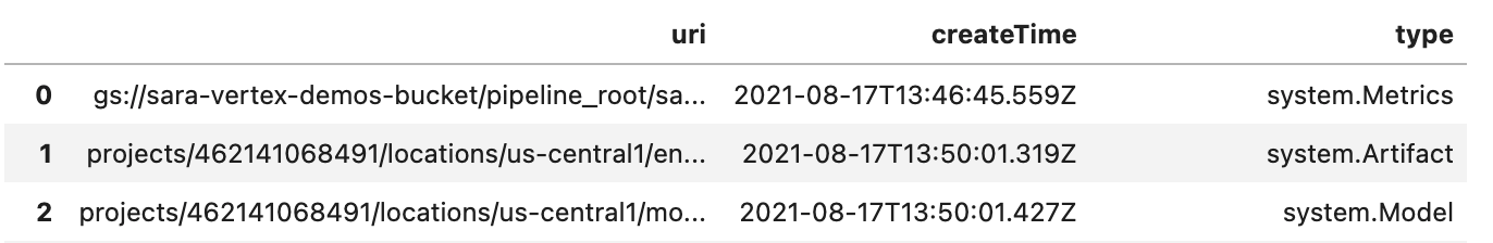
Affichez ensuite les résultats dans un DataFrame :

data = {'uri': [], 'createTime': [], 'type': []}

for i in live_artifacts:
    data['uri'].append(i.uri)
    data['createTime'].append(i.create_time)
    data['type'].append(i.schema_title)

df = pd.DataFrame.from_dict(data)
df

Le résultat qui s'affiche doit ressembler à ceci :

Vous pouvez également filtrer les artefacts en fonction d'autres critères que ceux que vous avez essayés ici.

Vous avez terminé l'atelier.

🎉 Félicitations ! 🎉

Vous savez désormais utiliser Vertex AI pour :

• Utiliser le SDK Kubeflow Pipelines pour créer un pipeline de ML qui crée un ensemble de données dans Vertex AI, puis entraîne et déploie un modèle Scikit-learn personnalisé sur cet ensemble de données
• Écrire des composants de pipeline personnalisés qui génèrent des artefacts et des métadonnées.
• Comparer les exécutions de Vertex Pipelines, dans la console Cloud et par programmation.
• Assurer la traçabilité des artefacts générés par le pipeline
• Interroger les métadonnées d'exécution du pipeline.

Pour en savoir plus sur les différents composants de Vertex, consultez la documentation.

9. Nettoyage

Pour éviter que des frais ne vous soient facturés, nous vous recommandons de supprimer les ressources créées tout au long de cet atelier.

Arrêter ou supprimer votre instance Notebooks

Si vous souhaitez continuer à utiliser le notebook que vous avez créé dans cet atelier, nous vous recommandons de le désactiver quand vous ne vous en servez pas. À partir de l'interface utilisateur de Notebooks dans la console Cloud, sélectionnez le notebook et cliquez sur Arrêter. Si vous souhaitez supprimer l'instance définitivement, sélectionnez Supprimer :

Supprimer vos points de terminaison Vertex AI

Pour supprimer le point de terminaison que vous avez déployé, accédez à la section Points de terminaison de votre console Vertex AI, puis cliquez sur l'icône de suppression :

Supprimer votre bucket Cloud Storage

Pour supprimer le bucket de stockage, utilisez le menu de navigation de la console Cloud pour accéder à Stockage, sélectionnez votre bucket puis cliquez sur "Supprimer" :