1. Descripción general
En este lab, aprenderás a usar Vertex AI Workbench para explorar datos y entrenar modelos de AA.
Qué aprenderá
Aprenderás a hacer lo siguiente:
- Crea y configura una instancia de Vertex AI Workbench
- Usa el conector de BigQuery de Vertex AI Workbench
- Entrena un modelo en un kernel de Vertex AI Workbench
El costo total de la ejecución de este lab en Google Cloud es de aproximadamente $1.
2. Introducción a Vertex AI
En este lab, se utiliza la oferta de productos de IA más reciente de Google Cloud. Vertex AI integra las ofertas de AA de Google Cloud en una experiencia de desarrollo fluida. Anteriormente, se podía acceder a los modelos personalizados y a los entrenados con AutoML mediante servicios independientes. La nueva oferta combina ambos en una sola API, junto con otros productos nuevos. También puedes migrar proyectos existentes a Vertex AI.
Vertex AI incluye muchos productos distintos para respaldar flujos de trabajo de AA de extremo a extremo. Este lab se enfocará en Vertex AI Workbench.
Vertex AI Workbench ayuda a los usuarios a compilar con rapidez flujos de trabajo basados en notebooks de extremo a extremo a través de la integración profunda a servicios de datos (como Dataproc, Dataflow, BigQuery y Dataplex) y Vertex AI. Además, permite a los científicos de datos conectarse a los servicios de datos de GCP, analizar conjuntos de datos, experimentar con diferentes técnicas de modelado, implementar los modelos entrenados en producción y administrar MLOps a lo largo del ciclo de vida del modelo.
3. Descripción general del caso de uso
En este lab, explorarás el conjunto de datos London Bicycles Hire. Estos datos contienen información sobre los viajes en bicicleta del programa público de uso compartido de bicicletas de Londres desde 2011. Comenzarás por explorar este conjunto de datos en BigQuery a través del conector de BigQuery de Vertex AI Workbench. Luego, cargarás los datos en un notebook de Jupyter con pandas y entrenarás un modelo de TensorFlow para predecir la duración de un viaje en bicicleta según cuándo ocurrió el viaje y la distancia que recorrió la persona en bicicleta.
En este lab, se usan las capas de procesamiento previo de Keras para transformar y preparar los datos de entrada para el entrenamiento del modelo. Esta API te permite compilar el procesamiento previo directamente en el grafo de tu modelo de TensorFlow, lo que reduce el riesgo de sesgo de entrenamiento o entrega, ya que garantiza que los datos de entrenamiento y los datos de entrega se sometan a transformaciones idénticas. Ten en cuenta que, a partir de TensorFlow 2.6, esta API es estable. Si usas una versión anterior de TensorFlow, deberás importar el símbolo experimental.
4. Configura el entorno
Para ejecutar este codelab, necesitarás un proyecto de Google Cloud Platform que tenga habilitada la facturación. Para crear un proyecto, sigue estas instrucciones.
Paso 1: Habilita la API de Compute Engine
Ve a Compute Engine y selecciona Habilitar (si aún no está habilitada).
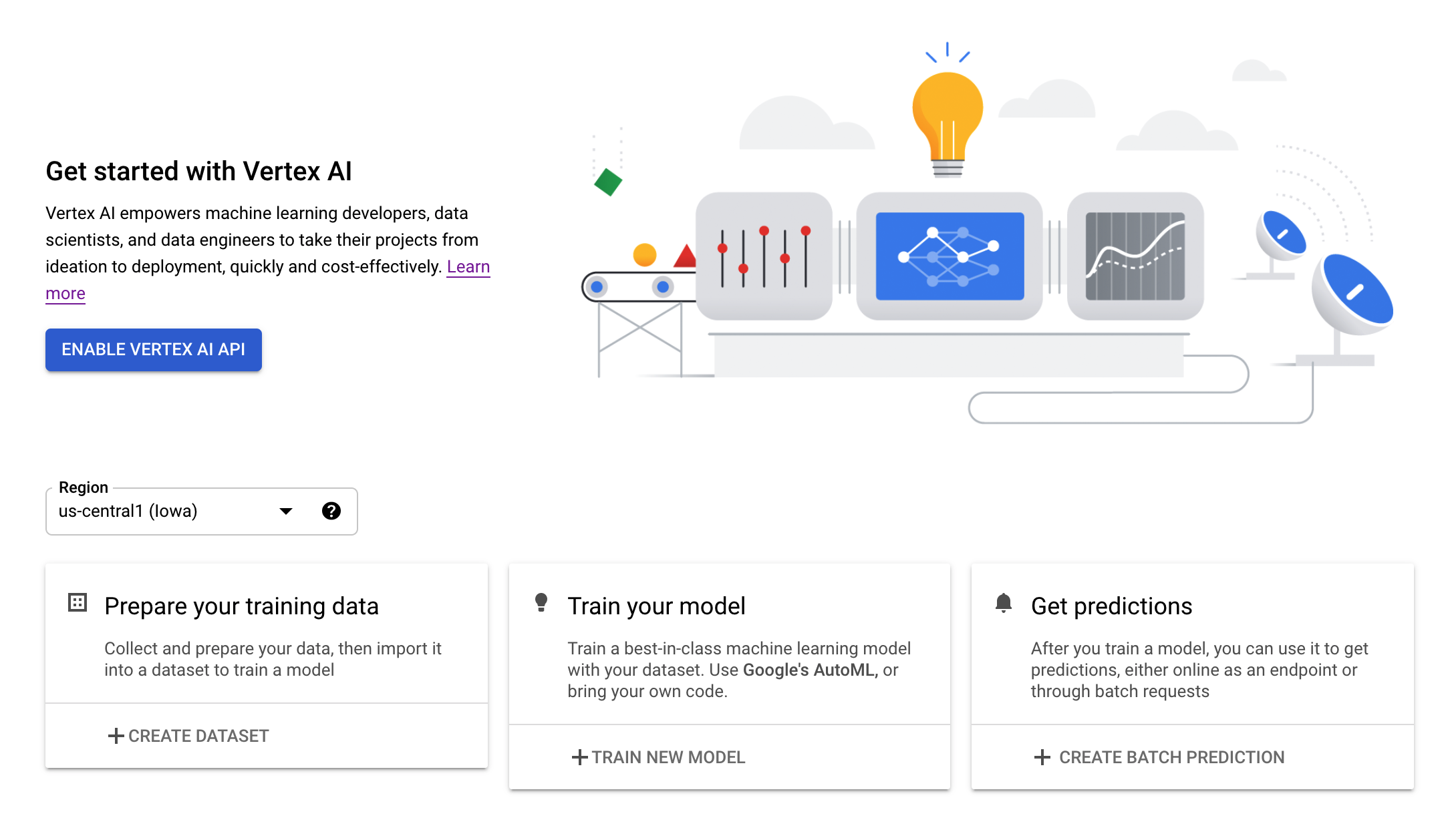
Paso 2: Habilita la API de Vertex AI
Navegue hasta la sección de Vertex AI en la consola de Cloud y haga clic en Habilitar API de Vertex AI.
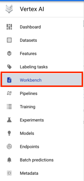
Paso 3: Crea una instancia de Vertex AI Workbench
En la sección Vertex AI de Cloud Console, haz clic en Workbench:
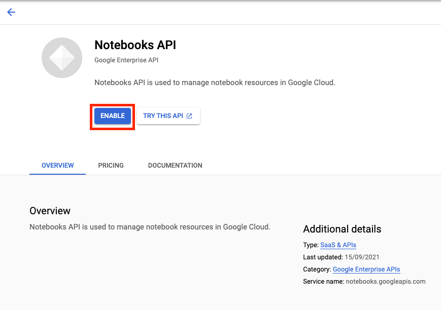
Habilita la API de Notebooks si aún no está habilitada.
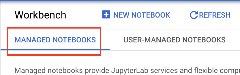
Una vez habilitada, haz clic en NOTEBOOKS ADMINISTRADOS (MANAGED NOTEBOOKS):
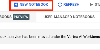
Luego, selecciona NUEVO NOTEBOOK (NEW NOTEBOOK).
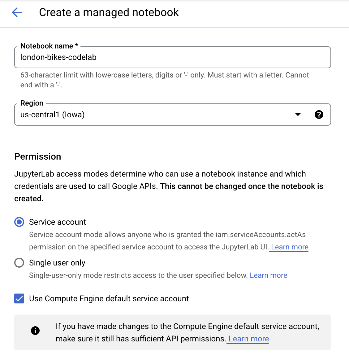
Asígnale un nombre al notebook y en Permiso (Permission), selecciona Cuenta de servicio (Service account).
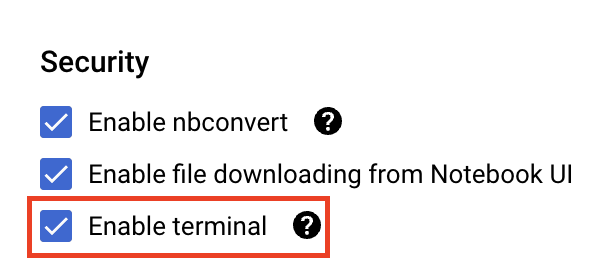
Selecciona Configuración avanzada.
En Seguridad (Security), selecciona la opción “Habilitar terminal” (Enable terminal) si aún no está habilitada.
Puedes dejar el resto de la configuración avanzada tal como está.
Luego, haz clic en Crear.
Una vez que se cree la instancia, selecciona ABRIR JUPYTERLAB (OPEN JUPYTERLAB).

5. Explora el conjunto de datos en BigQuery
En la instancia de Vertex AI Workbench, navega al lado izquierdo y haz clic en el conector BigQuery en notebooks.
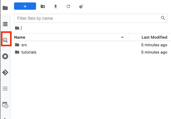
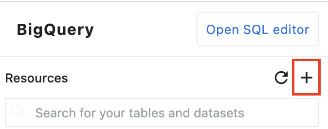
El conector de BigQuery te permite explorar y consultar conjuntos de datos de BigQuery con facilidad. Además de los conjuntos de datos de tu proyecto, puedes explorar conjuntos de datos de otros proyectos haciendo clic en el botón Agregar proyecto.
En este lab, usarás datos de los conjuntos de datos públicos de BigQuery. Desplázate hacia abajo hasta encontrar el conjunto de datos london_bicycles. Verás que este conjunto de datos tiene dos tablas, cycle_hire y cycle_stations. Exploremos cada una de ellas.

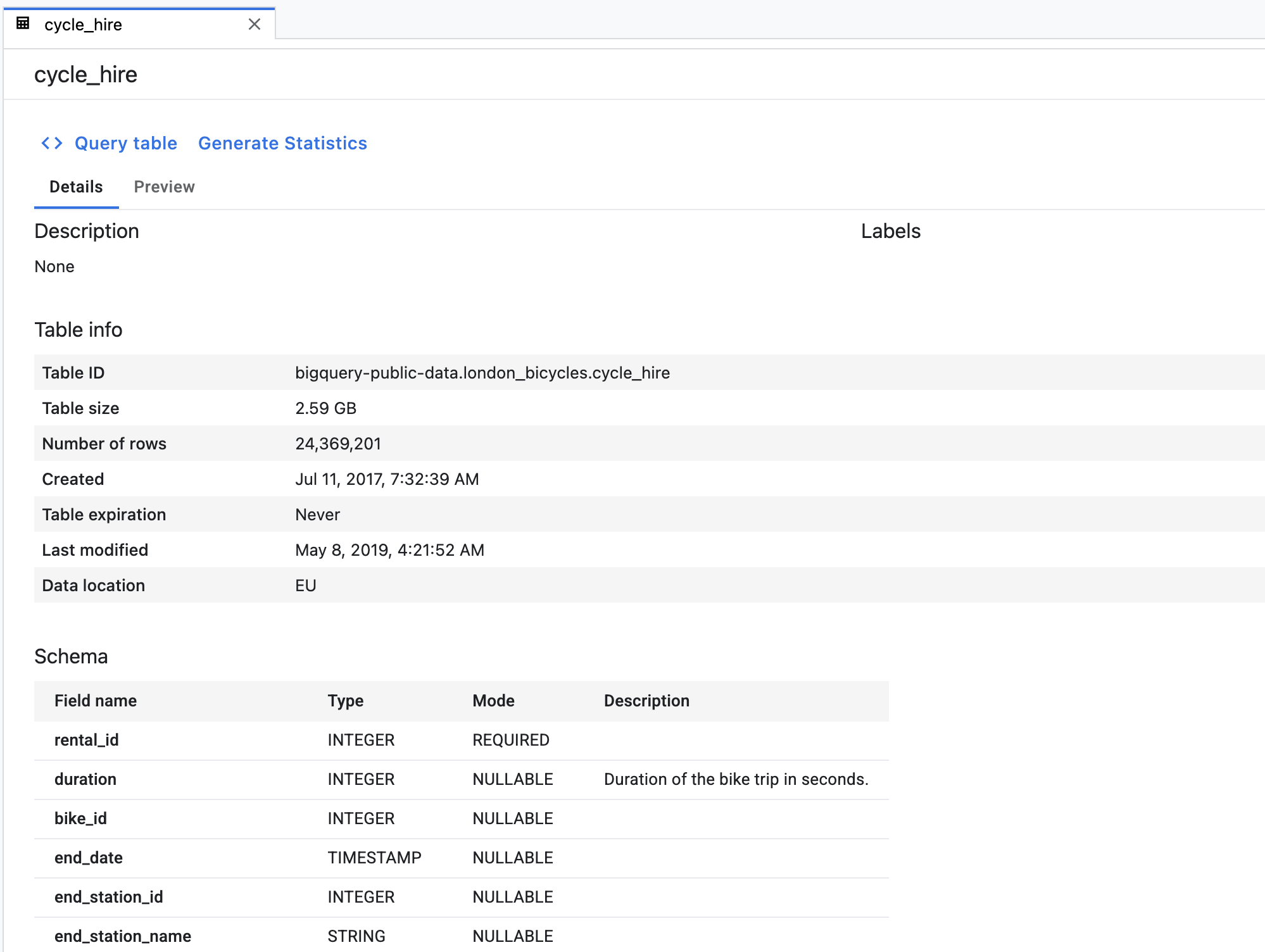
Primero, haz doble clic en la tabla cycle_hire. Verás que la tabla se abre como una pestaña nueva con el esquema de la tabla, así como metadatos como la cantidad de filas y el tamaño.
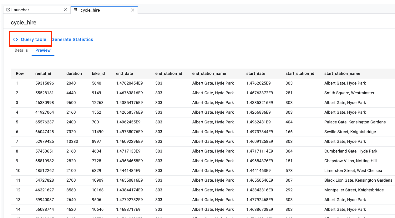
Si haces clic en la pestaña Vista previa, podrás ver una muestra de los datos. Vamos a ejecutar una consulta simple para ver cuáles son los recorridos populares. Primero, haz clic en el botón Consultar tabla.
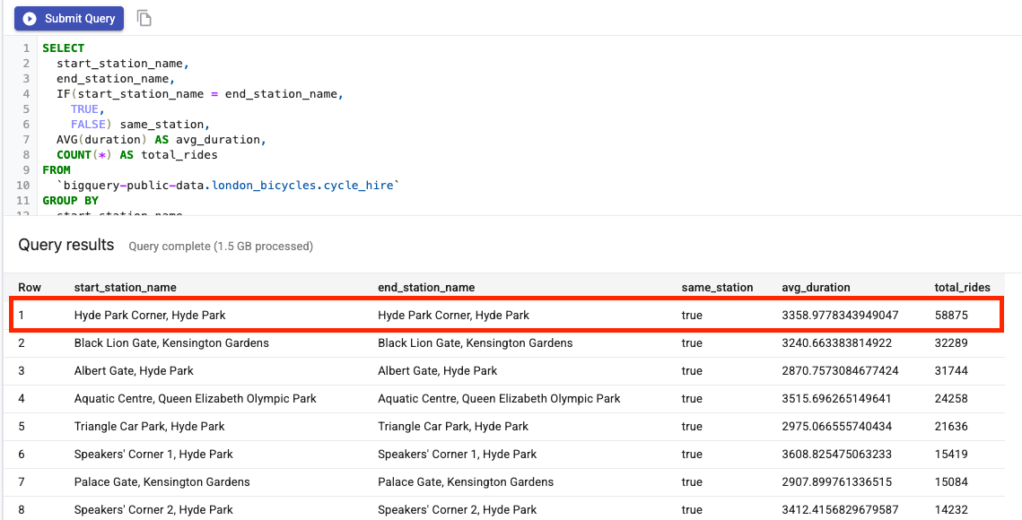
Luego, pega lo siguiente en el editor de SQL y haz clic en Enviar consulta.
SELECT
  start_station_name,
  end_station_name,
  IF(start_station_name = end_station_name,
    TRUE,
    FALSE) same_station,
  AVG(duration) AS avg_duration,
  COUNT(*) AS total_rides
FROM
  `bigquery-public-data.london_bicycles.cycle_hire`
GROUP BY
  start_station_name,
  end_station_name,
  same_station
ORDER BY
  total_rides DESC
En los resultados de la consulta, verás que los viajes en bicicleta hacia y desde la estación Hyde Park Corner fueron los más populares.
A continuación, haz doble clic en la tabla cycle_stations, que proporciona información sobre cada estación.
Queremos unir las tablas cycle_hire y cycle_stations. La tabla cycle_stations contiene la latitud y longitud de cada estación. Usarás esta información para calcular la distancia recorrida en cada viaje en bicicleta calculando la distancia entre las estaciones de inicio y destino.
Para realizar este cálculo, usarás las funciones geográficas de BigQuery. Específicamente, convertirás cada cadena de lat/lon en un ST_GEOGPOINT y usarás la función ST_DISTANCE para calcular la distancia en línea recta en metros entre los dos puntos. Utilizarás este valor como un proxy de la distancia recorrida en cada viaje en bicicleta.
Copia la siguiente consulta en tu editor de SQL y, luego, haz clic en Enviar consulta. Ten en cuenta que hay tres tablas en la condición JOIN porque debemos unir la tabla de estaciones dos veces para obtener la latitud y longitud de la estación de partida y de finalización del ciclo.
WITH staging AS (
    SELECT
        STRUCT(
            start_stn.name,
            ST_GEOGPOINT(start_stn.longitude, start_stn.latitude) AS POINT,
            start_stn.docks_count,
            start_stn.install_date
        ) AS starting,
        STRUCT(
            end_stn.name,
            ST_GEOGPOINT(end_stn.longitude, end_stn.latitude) AS point,
            end_stn.docks_count,
            end_stn.install_date
        ) AS ending,
        STRUCT(
            rental_id,
            bike_id,
            duration, --seconds
            ST_DISTANCE(
                ST_GEOGPOINT(start_stn.longitude, start_stn.latitude),
                ST_GEOGPOINT(end_stn.longitude, end_stn.latitude)
            ) AS distance, --meters
            start_date,
            end_date
        ) AS bike
        FROM `bigquery-public-data.london_bicycles.cycle_stations` AS start_stn
        LEFT JOIN `bigquery-public-data.london_bicycles.cycle_hire` as b
        ON start_stn.id = b.start_station_id
        LEFT JOIN `bigquery-public-data.london_bicycles.cycle_stations` AS end_stn
        ON end_stn.id = b.end_station_id
        LIMIT 700000)

SELECT * from STAGING
6. Entrena un modelo de AA en un kernel de TensorFlow
Vertex AI Workbench tiene una capa de compatibilidad de procesamiento que te permite iniciar kernels para TensorFlow, PySpark, R, etcétera, todo desde una sola instancia de notebook. En este lab, crearás un notebook con el kernel de TensorFlow.
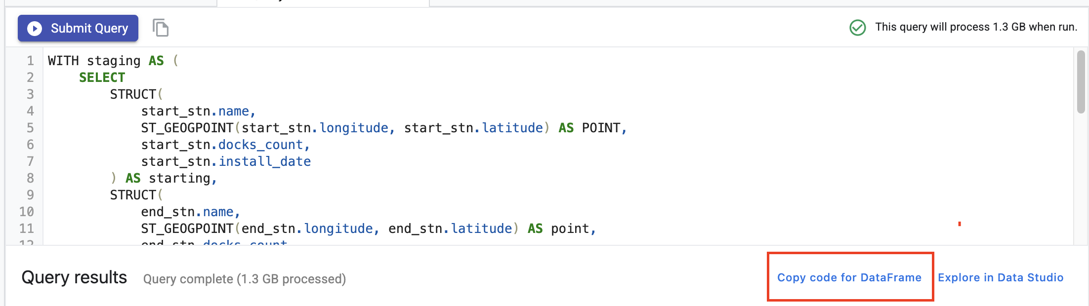
Crear DataFrame
Una vez ejecutada la consulta, haz clic en Copiar código para DataFrame. Esto te permitirá pegar el código de Python en un notebook que se conecta con el cliente de BigQuery y extrae estos datos como un DataFrame de Pandas.
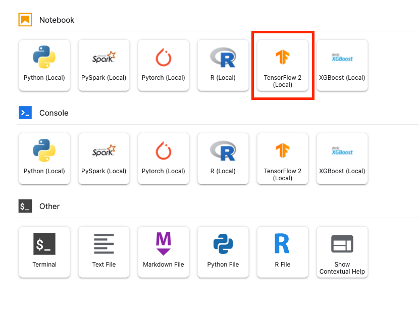
A continuación, regresa al selector y crea un notebook de TensorFlow 2.
En la primera celda del notebook, pega el código copiado del editor de consultas. Debería verse de la siguiente manera:
# The following two lines are only necessary to run once.
# Comment out otherwise for speed-up.
from google.cloud.bigquery import Client, QueryJobConfig
client = Client()

query = """WITH staging AS (
    SELECT
        STRUCT(
            start_stn.name,
            ST_GEOGPOINT(start_stn.longitude, start_stn.latitude) AS POINT,
            start_stn.docks_count,
            start_stn.install_date
        ) AS starting,
        STRUCT(
            end_stn.name,
            ST_GEOGPOINT(end_stn.longitude, end_stn.latitude) AS point,
            end_stn.docks_count,
            end_stn.install_date
        ) AS ending,
        STRUCT(
            rental_id,
            bike_id,
            duration, --seconds
            ST_DISTANCE(
                ST_GEOGPOINT(start_stn.longitude, start_stn.latitude),
                ST_GEOGPOINT(end_stn.longitude, end_stn.latitude)
            ) AS distance, --meters
            start_date,
            end_date
        ) AS bike
        FROM `bigquery-public-data.london_bicycles.cycle_stations` AS start_stn
        LEFT JOIN `bigquery-public-data.london_bicycles.cycle_hire` as b
        ON start_stn.id = b.start_station_id
        LEFT JOIN `bigquery-public-data.london_bicycles.cycle_stations` AS end_stn
        ON end_stn.id = b.end_station_id
        LIMIT 700000)

SELECT * from STAGING"""
job = client.query(query)
df = job.to_dataframe()
A los efectos de este lab, limitamos el conjunto de datos a 700,000 para acortar el tiempo de entrenamiento. Sin embargo, no dudes en modificar la consulta y experimentar con todo el conjunto de datos.
A continuación, importa las bibliotecas necesarias.
from datetime import datetime
import pandas as pd
import tensorflow as tf
Ejecuta el siguiente código para crear un DataFrame reducido que solo contenga las columnas necesarias para la parte de AA de este ejercicio.
values = df['bike'].values
duration = list(map(lambda a: a['duration'], values))
distance = list(map(lambda a: a['distance'], values))
dates = list(map(lambda a: a['start_date'], values))
data = pd.DataFrame(data={'duration': duration, 'distance': distance, 'start_date':dates})
data = data.dropna()
La columna start_date es un datetime de Python. En lugar de usar este datetime directamente en el modelo, crearás dos atributos nuevos que indiquen el día de la semana y la hora del día en que ocurrió el viaje en bicicleta.
data['weekday'] = data['start_date'].apply(lambda a: a.weekday())
data['hour'] = data['start_date'].apply(lambda a: a.time().hour)
data = data.drop(columns=['start_date'])
Por último, convierte la columna de duración de segundos a minutos para que sea más fácil de entender.
data['duration'] = data['duration'].apply(lambda x:float(x / 60))
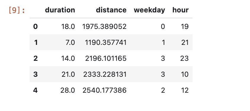
Examina las primeras filas del DataFrame con formato. Para cada viaje en bicicleta, ahora tienes datos sobre el día de la semana y la hora del día en que se realizó el viaje, así como la distancia recorrida. Con esta información, intentarás predecir cuánto tiempo tardó el viaje.
data.head()
Antes de crear y entrenar el modelo, debes dividir los datos en conjuntos de entrenamiento y validación.
# Use 80/20 train/eval split
train_size = int(len(data) * .8)
print ("Train size: %d" % train_size)
print ("Evaluation size: %d" % (len(data) - train_size))

# Split data into train and test sets
train_data = data[:train_size]
val_data = data[train_size:]
Crear un modelo de TensorFlow
Crearás un modelo de TensorFlow con la API funcional de Keras. Para procesar previamente los datos de entrada, usarás la API de capas de procesamiento previo de Keras.
La siguiente función de utilidad creará un tf.data.Dataset a partir del DataFrame de pandas.
def df_to_dataset(dataframe, label, shuffle=True, batch_size=32):
  dataframe = dataframe.copy()
  labels = dataframe.pop(label)
  ds = tf.data.Dataset.from_tensor_slices((dict(dataframe), labels))
  if shuffle:
    ds = ds.shuffle(buffer_size=len(dataframe))
  ds = ds.batch(batch_size)
  ds = ds.prefetch(batch_size)
  return ds
Usa la función anterior para crear dos tf.data.Dataset, uno para el entrenamiento y otro para la validación. Es posible que veas algunas advertencias, pero puedes ignorarlas de forma segura.
train_dataset = df_to_dataset(train_data, 'duration')
validation_dataset = df_to_dataset(val_data, 'duration')
Usarás las siguientes capas de procesamiento previo en el modelo:
- Capa de normalización: realiza la normalización de los atributos de entrada.
- Capa de IntegerLookup: convierte los valores categóricos de números enteros en índices de números enteros.
- Capa CategoryEncoding: Convierte los atributos categóricos de números enteros en representaciones densas one-hot, multi-hot o TF-IDF.
Ten en cuenta que estas capas no se pueden entrenar. En su lugar, configuras el estado de la capa de procesamiento previo exponiéndola a los datos de entrenamiento a través del método adapt().
La siguiente función creará una capa de normalización que puedes usar en el componente distancia. Para establecer el estado antes de ajustar el modelo, usarás el método adapt() en los datos de entrenamiento. Esto calculará la media y la varianza que se usarán para la normalización. Más adelante, cuando pases el conjunto de datos de validación al modelo, se usarán esta misma media y varianza calculadas en los datos de entrenamiento para escalar los datos de validación.
def get_normalization_layer(name, dataset):
  # Create a Normalization layer for our feature.
  normalizer = tf.keras.layers.Normalization(axis=None)

  # Prepare a Dataset that only yields our feature.
  feature_ds = dataset.map(lambda x, y: x[name])

  # Learn the statistics of the data.
  normalizer.adapt(feature_ds)

  return normalizer
De manera similar, la siguiente función crea una codificación de categoría que usarás en las funciones de hora y día de la semana.
def get_category_encoding_layer(name, dataset, dtype, max_tokens=None):
  index = tf.keras.layers.IntegerLookup(max_tokens=max_tokens)

  # Prepare a Dataset that only yields our feature
  feature_ds = dataset.map(lambda x, y: x[name])

  # Learn the set of possible values and assign them a fixed integer index.
  index.adapt(feature_ds)

  # Create a Discretization for our integer indices.
  encoder = tf.keras.layers.CategoryEncoding(num_tokens=index.vocabulary_size())

  # Apply one-hot encoding to our indices. The lambda function captures the
  # layer so we can use them, or include them in the functional model later.
  return lambda feature: encoder(index(feature))
A continuación, crea la parte de procesamiento previo del modelo. Primero, crea una capa tf.keras.Input para cada uno de los componentes.
# Create a Keras input layer for each feature
numeric_col = tf.keras.Input(shape=(1,), name='distance')
hour_col = tf.keras.Input(shape=(1,), name='hour', dtype='int64')
weekday_col = tf.keras.Input(shape=(1,), name='weekday', dtype='int64')
Luego, crea las capas de normalización y codificación de categorías y almacénalas en una lista.
all_inputs = []
encoded_features = []

# Pass 'distance' input to normalization layer
normalization_layer = get_normalization_layer('distance', train_dataset)
encoded_numeric_col = normalization_layer(numeric_col)
all_inputs.append(numeric_col)
encoded_features.append(encoded_numeric_col)

# Pass 'hour' input to category encoding layer
encoding_layer = get_category_encoding_layer('hour', train_dataset, dtype='int64')
encoded_hour_col = encoding_layer(hour_col)
all_inputs.append(hour_col)
encoded_features.append(encoded_hour_col)

# Pass 'weekday' input to category encoding layer
encoding_layer = get_category_encoding_layer('weekday', train_dataset, dtype='int64')
encoded_weekday_col = encoding_layer(weekday_col)
all_inputs.append(weekday_col)
encoded_features.append(encoded_weekday_col)
Después de definir las capas de procesamiento previo, puedes definir el resto del modelo. Concatenarás todas las funciones de entrada y las pasarás a una capa densa. La capa de salida es una sola unidad, ya que este es un problema de regresión.
all_features = tf.keras.layers.concatenate(encoded_features)
x = tf.keras.layers.Dense(64, activation="relu")(all_features)
output = tf.keras.layers.Dense(1)(x)
model = tf.keras.Model(all_inputs, output)
Por último, compila el modelo.
model.compile(optimizer = tf.keras.optimizers.Adam(0.001),
              loss='mean_squared_logarithmic_error')
Ahora que definiste el modelo, puedes visualizar la arquitectura
tf.keras.utils.plot_model(model, show_shapes=True, rankdir="LR")
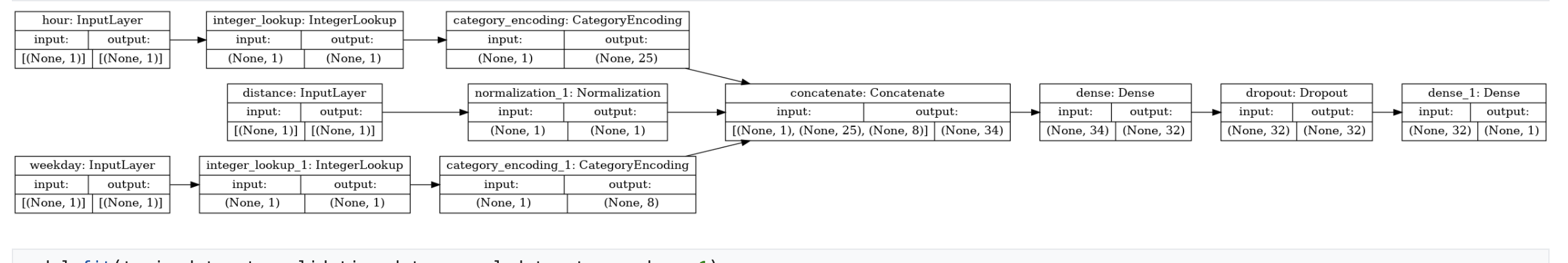
Ten en cuenta que este modelo es bastante complicado para este conjunto de datos simple. Se diseñó con fines de demostración.
Entrenémoslo durante 1 ciclo de entrenamiento solo para confirmar que se ejecute el código.
model.fit(train_dataset, validation_data = validation_dataset, epochs = 1)
Entrena el modelo con una GPU
A continuación, entrenarás el modelo por más tiempo y usarás el conmutador de hardware para acelerar el entrenamiento. Vertex AI Workbench te permite cambiar el hardware sin cerrar la instancia. Si agregas la GPU solo cuando la necesitas, puedes mantener los costos bajos.
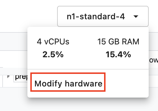
Para cambiar el perfil de hardware, haz clic en el tipo de máquina en la esquina superior derecha y selecciona Modificar hardware.
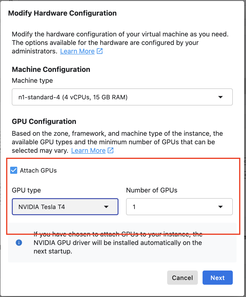
Selecciona Attach GPUs y, luego, una GPU NVIDIA T4 Tensor Core.
El hardware tardará unos cinco minutos en configurarse. Una vez que se complete el proceso, entrenemos el modelo un poco más. Notarás que cada época ahora lleva menos tiempo.
model.fit(train_dataset, validation_data = validation_dataset, epochs = 5)
🎉 ¡Felicitaciones! 🎉
Aprendiste a usar Vertex AI Workbench para hacer lo siguiente:
- Explora datos en BigQuery
- Usa el cliente de BigQuery para cargar datos en Python
- Entrena un modelo de TensorFlow con capas de procesamiento previo de Keras y una GPU
Si quieres obtener más información sobre los diferentes componentes de Vertex AI, consulta la documentación.
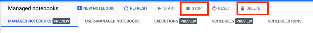
7. Realiza una limpieza
Debido a que configuramos el notebook para que se agote el tiempo de espera después de 60 minutos de inactividad, no tenemos que preocuparnos por cerrar la instancia. Si quieres cerrar la instancia de forma manual, haz clic en el botón Detener (Stop) en la sección Vertex AI Workbench de la consola. Si quieres borrar el notebook por completo, haz clic en el botón Borrar (Delete).