
1. Overview
This tutorial has been updated for Tensorflow 2.2 !
In this codelab, you will learn how to build and train a neural network that recognises handwritten digits. Along the way, as you enhance your neural network to achieve 99% accuracy, you will also discover the tools of the trade that deep learning professionals use to train their models efficiently.
This codelab uses the MNIST dataset, a collection of 60,000 labeled digits that has kept generations of PhDs busy for almost two decades. You will solve the problem with less than 100 lines of Python / TensorFlow code.
What you'll learn
- What is a neural network and how to train it
- How to build a basic 1-layer neural network using tf.keras
- How to add more layers
- How to set up a learning rate schedule
- How to build convolutional neural networks
- How to use regularisation techniques: dropout, batch normalization
- What is overfitting
What you'll need
Just a browser. This workshop can be run entirely with Google Colaboratory.
Feedback
Please tell us if you see something amiss in this lab or if you think it should be improved. We handle feedback through GitHub issues [ feedback link].
2. Google Colaboratory quick start
This lab uses Google Colaboratory and requires no setup on your part. You can run it from a Chromebook. Please open the file below, and execute the cells to familiarize yourself with Colab notebooks.

Additional instructions below:
Select a GPU backend

In the Colab menu, select Runtime > Change runtime type and then select GPU. Connection to the runtime will happen automatically on first execution, or you can use the "Connect" button in the upper-right corner.
Notebook execution
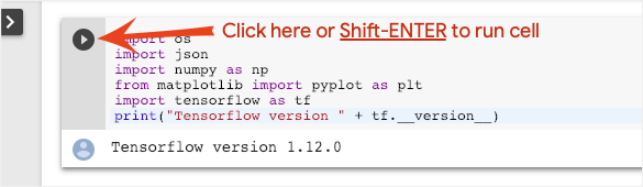
Execute cells one at a time by clicking on a cell and using Shift-ENTER. You can also run the entire notebook with Runtime > Run all
Table of contents

All notebooks have a table of contents. You can open it using the black arrow on the left.
Hidden cells

Some cells will only show their title. This is a Colab-specific notebook feature. You can double click on them to see the code inside but it is usually not very interesting. Typically support or visualization functions. You still need to run these cells for the functions inside to be defined.
3. Train a neural network
We will first watch a neural network train. Please open the notebook below and run through all the cells. Do not pay attention to the code yet, we will start explaining it later.
As you execute the notebook, focus on the visualizations. See below for explanations.
Training data
We have a dataset of handwritten digits which have been labeled so that we know what each picture represents, i.e. a number between 0 and 9. In the notebook, you will see an excerpt:
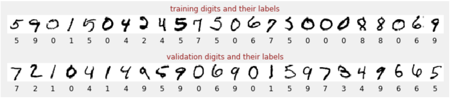
The neural network we will build classifies the handwritten digits in their 10 classes (0, .., 9). It does so based on internal parameters that need to have a correct value for the classification to work well. This "correct value" is learned through a training process which requires a "labeled dataset" with images and the associated correct answers.
How do we know if the trained neural network performs well or not? Using the training dataset to test the network would be cheating. It has already seen that dataset multiple times during training and is most certainly very performant on it. We need another labeled dataset, never seen during training, to evaluate the "real-world" performance of the network. It is called an "validation dataset"
Training
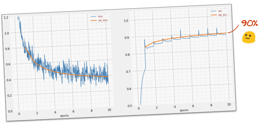
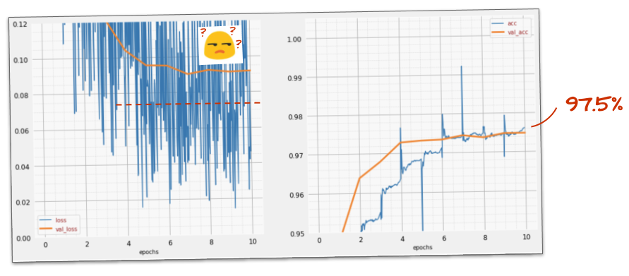
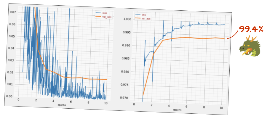
As training progresses, one batch of training data at a time, internal model parameters get updated and the model gets better and better at recognizing the handwritten digits. You can see it on the training graph:
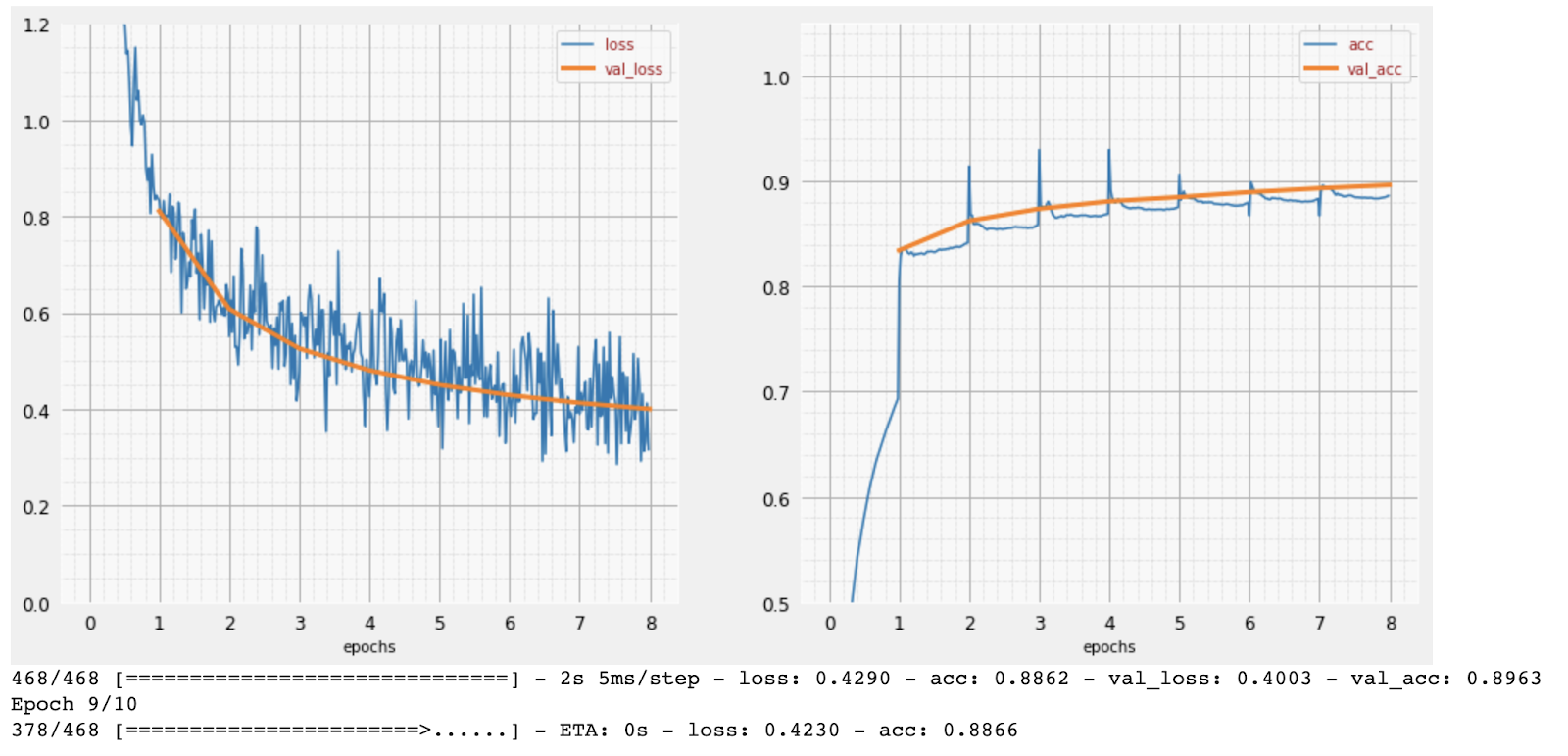
On the right, the "accuracy" is simply the percentage of correctly recognized digits. It goes up as training progresses, which is good.
On the left, we can see the "loss". To drive the training, we will define a "loss" function, which represents how badly the system recognises the digits, and try to minimise it. What you see here is that the loss goes down on both the training and the validation data as the training progresses: that is good. It means the neural network is learning.
The X-axis represents the number of "epochs" or iterations through the entire dataset.
Predictions
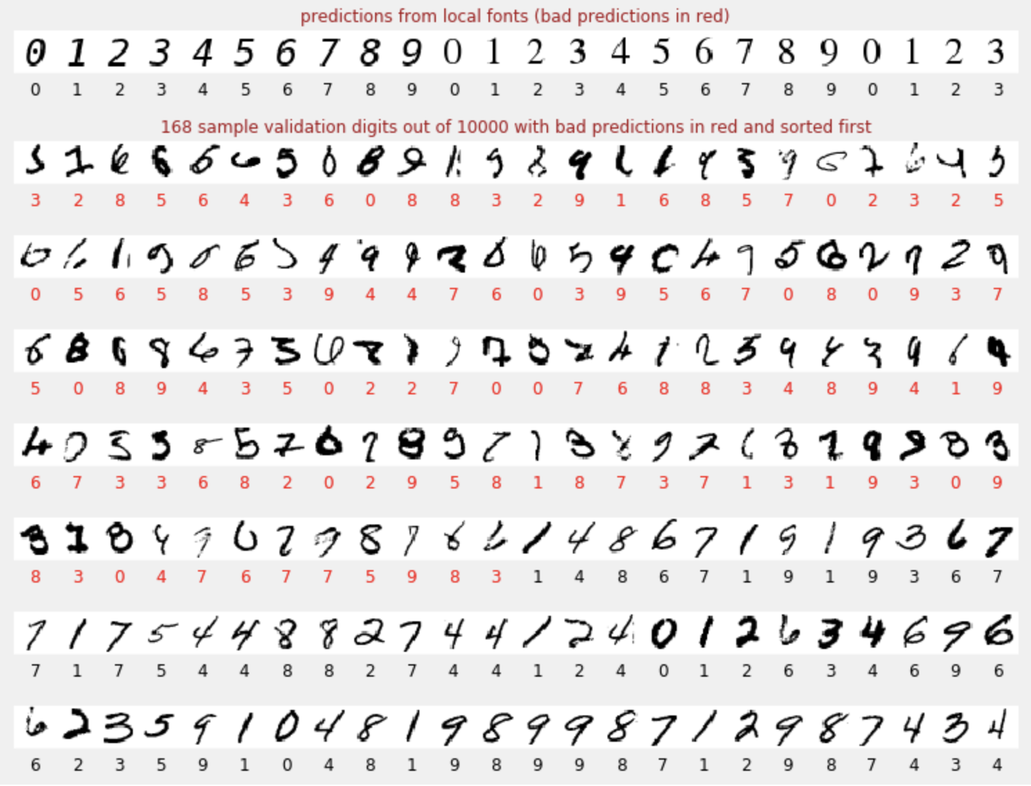
When the model is trained, we can use it to recognize handwritten digits. The next visualization shows how well it performs on a few digits rendered from local fonts (first line) and then on the 10,000 digits of the validation dataset. The predicted class appears under each digit, in red if it was wrong.
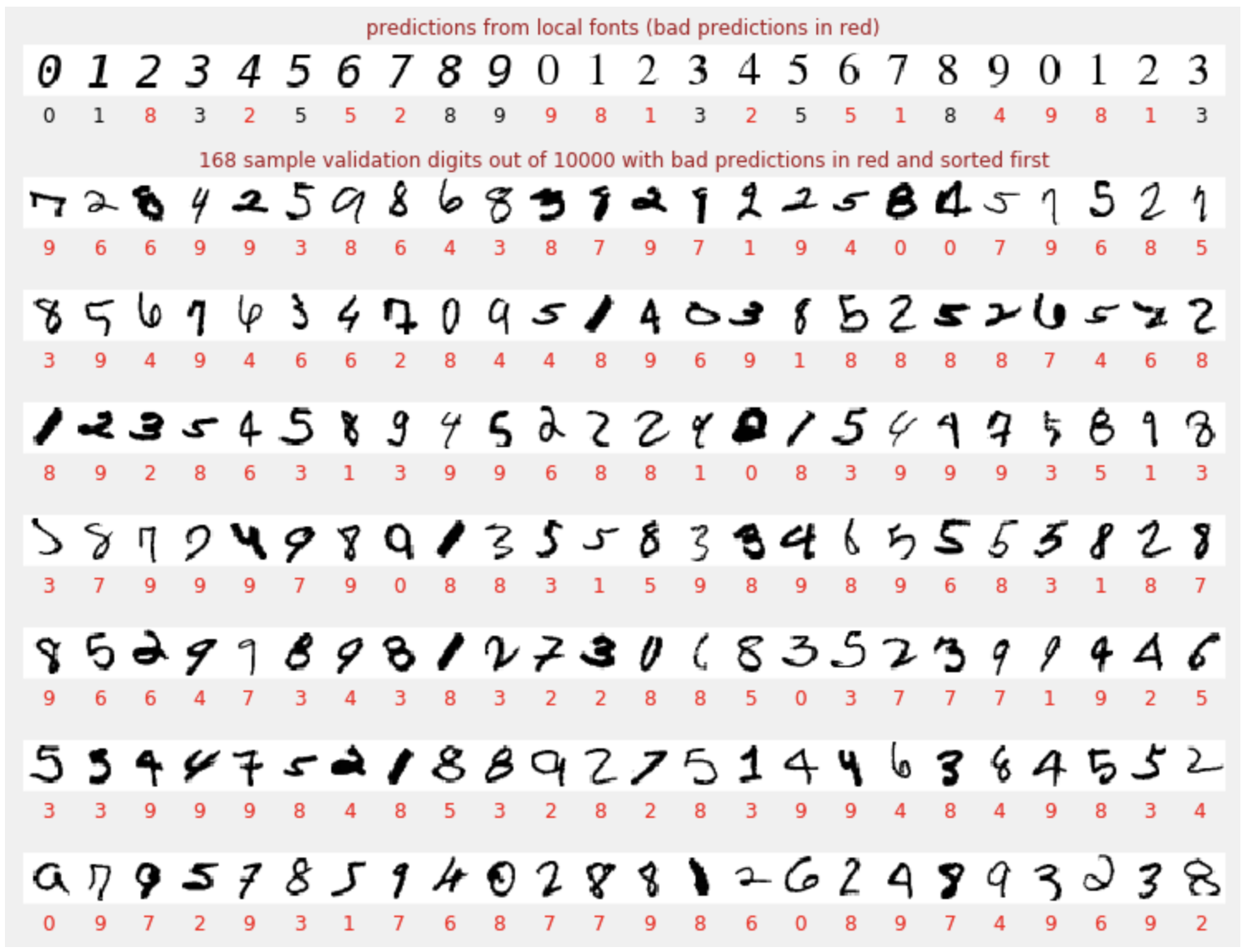
As you can see, this initial model is not very good but still recognizes some digits correctly. Its final validation accuracy is around 90% which is not so bad for the simplistic model we are starting with, but it still means that it misses 1000 validation digits out of the 10,000. That is far more that can be displayed, which is why it looks like all the answers are wrong (red).
Tensors
Data is stored in matrices. A 28x28 pixel grayscale image fits into a 28x28 two-dimensional matrix. But for a color image, we need more dimensions. There are 3 color values per pixel (Red, Green, Blue), so a three-dimensional table will be needed with dimensions [28, 28, 3]. And to store a batch of 128 color images, a four-dimensional table is needed with dimensions [128, 28, 28, 3].
These multi-dimensional tables are called "tensors" and the list of their dimensions is their "shape".
4. [INFO]: neural networks 101
In a nutshell
If all the terms in bold in the next paragraph are already known to you, you can move to the next exercise. If your are just starting in deep learning then welcome, and please read on.

For models built as a sequence of layers Keras offers the Sequential API. For example, an image classifier using three dense layers can be written in Keras as:
model = tf.keras.Sequential([
    tf.keras.layers.Flatten(input_shape=[28, 28, 1]),
    tf.keras.layers.Dense(200, activation="relu"),
    tf.keras.layers.Dense(60, activation="relu"),
    tf.keras.layers.Dense(10, activation='softmax') # classifying into 10 classes
])

# this configures the training of the model. Keras calls it "compiling" the model.
model.compile(
  optimizer='adam',
  loss= 'categorical_crossentropy',
  metrics=['accuracy']) # % of correct answers

# train the model
model.fit(dataset, ... )

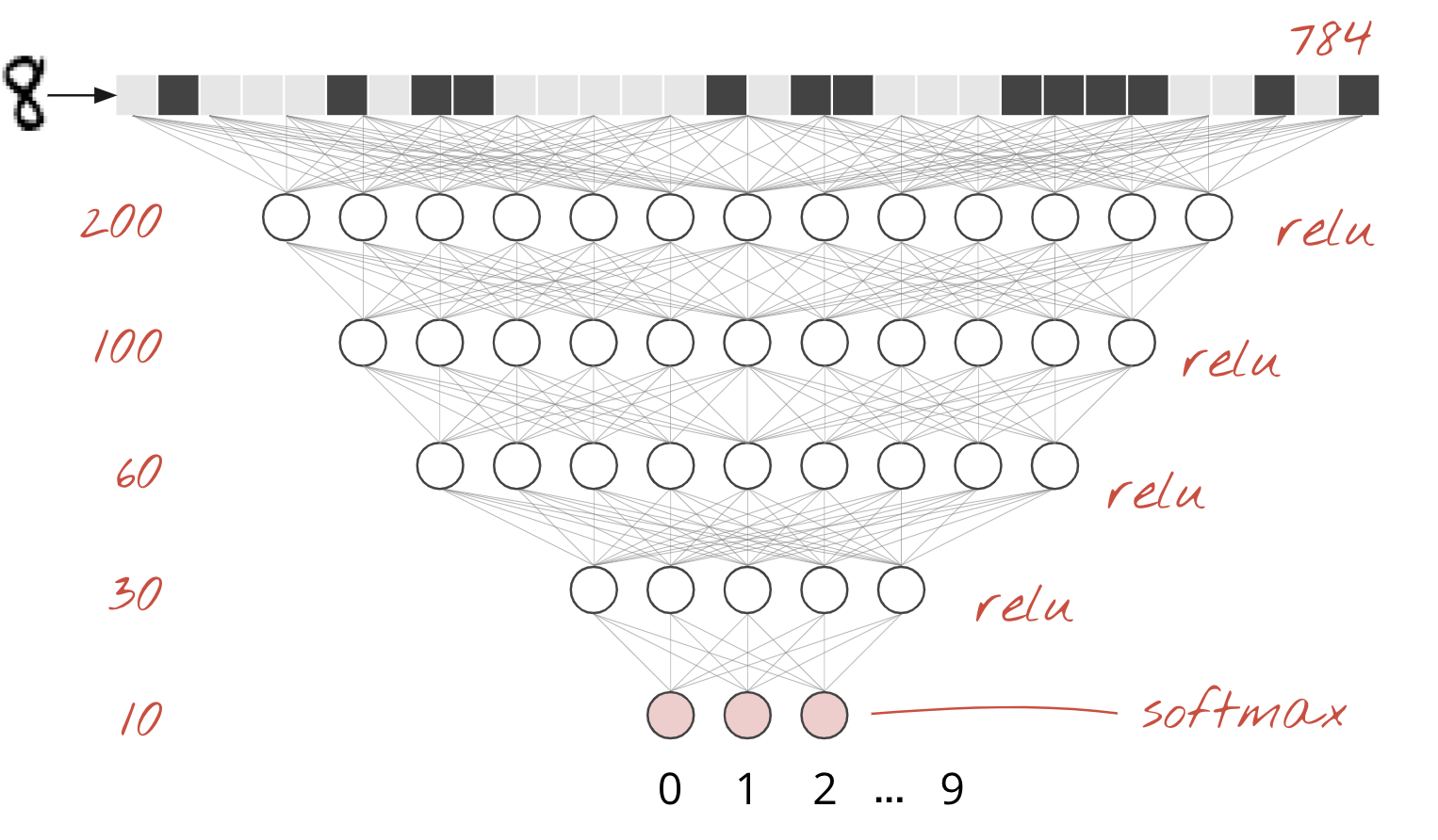
A single dense layer
Handwritten digits in the MNIST dataset are 28x28 pixel grayscale images. The simplest approach for classifying them is to use the 28x28=784 pixels as inputs for a 1-layer neural network.
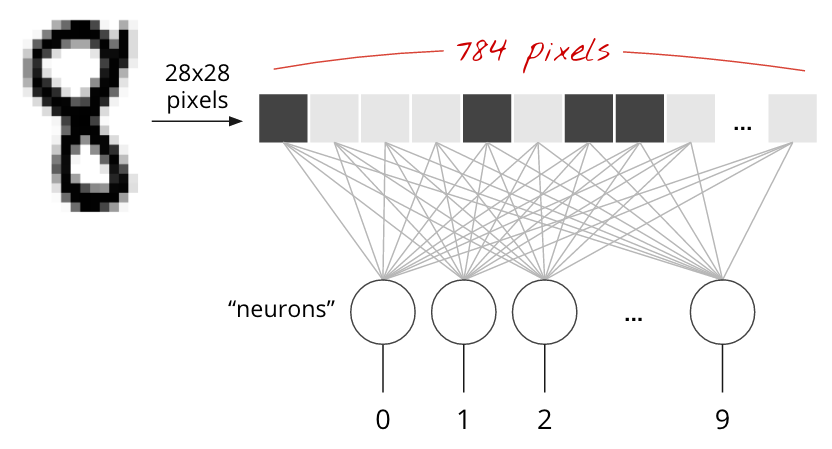
Each "neuron" in a neural network does a weighted sum of all of its inputs, adds a constant called the "bias" and then feeds the result through some non-linear "activation function". The "weights" and "biases" are parameters that will be determined through training. They are initialized with random values at first.
The picture above represents a 1-layer neural network with 10 output neurons since we want to classify digits into 10 classes (0 to 9).
With a matrix multiplication
Here is how a neural network layer, processing a collection of images, can be represented by a matrix multiplication:
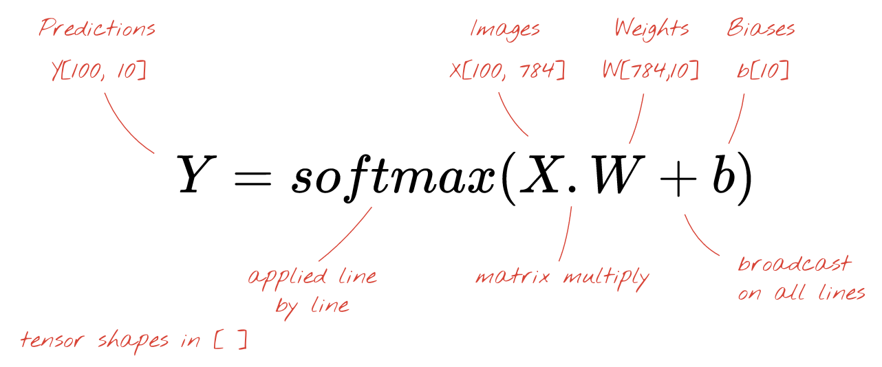
Using the first column of weights in the weights matrix W, we compute the weighted sum of all the pixels of the first image. This sum corresponds to the first neuron. Using the second column of weights, we do the same for the second neuron and so on until the 10th neuron. We can then repeat the operation for the remaining 99 images. If we call X the matrix containing our 100 images, all the weighted sums for our 10 neurons, computed on 100 images are simply X.W, a matrix multiplication.
Each neuron must now add its bias (a constant). Since we have 10 neurons, we have 10 bias constants. We will call this vector of 10 values b. It must be added to each line of the previously computed matrix. Using a bit of magic called "broadcasting" we will write this with a simple plus sign.
We finally apply an activation function, for example "softmax" (explained below) and obtain the formula describing a 1-layer neural network, applied to 100 images:
In Keras
With high-level neural network libraries like Keras, we will not need to implement this formula. However, it is important to understand that a neural network layer is just a bunch of multiplications and additions. In Keras, a dense layer would be written as:
tf.keras.layers.Dense(10, activation='softmax')
Go deep
It is trivial to chain neural network layers. The first layer computes weighted sums of of pixels. Subsequent layers compute weighted sums of the outputs of the previous layers.
The only difference, apart from the number of neurons, will be the choice of activation function.
Activation functions: relu, softmax and sigmoid
You would typically use the "relu" activation function for all layers but the last. The last layer, in a classifier, would use "softmax" activation.
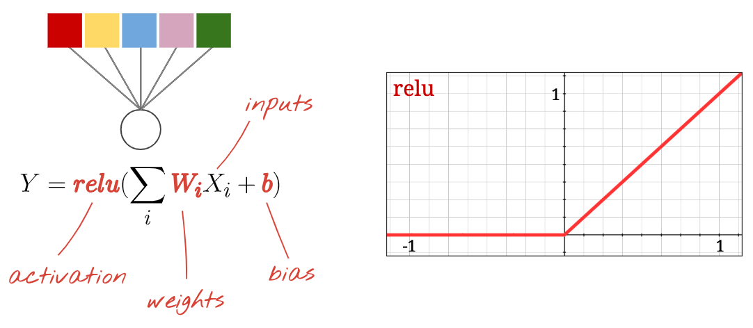
Again, a "neuron" computes a weighted sum of all of its inputs, adds a value called "bias" and feeds the result through the activation function.
The most popular activation function is called "RELU" for Rectified Linear Unit. It is a very simple function as you can see on the graph above.
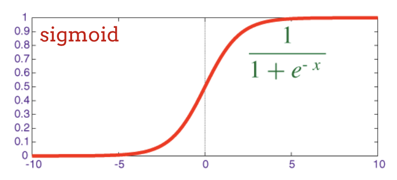
The traditional activation function in neural networks was the "sigmoid" but the "relu" was shown to have better convergence properties almost everywhere and is now preferred.
Softmax activation for classification
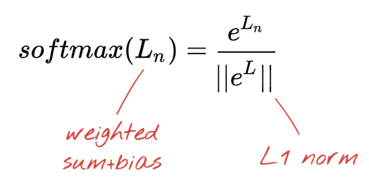
The last layer of our neural network has 10 neurons because we want to classify handwritten digits into 10 classes (0,..9). It should output 10 numbers between 0 and 1 representing the probability of this digit being a 0, a 1, a 2 and so on. For this, on the last layer, we will use an activation function called "softmax".
Applying softmax on a vector is done by taking the exponential of each element and then normalising the vector, typically by dividing it by its "L1" norm (i.e. sum of absolute values) so that normalized values add up to 1 and can be interpreted as probabilities.
The output of the last layer, before activation is sometimes called "logits". If this vector is L = [L0, L1, L2, L3, L4, L5, L6, L7, L8, L9], then:
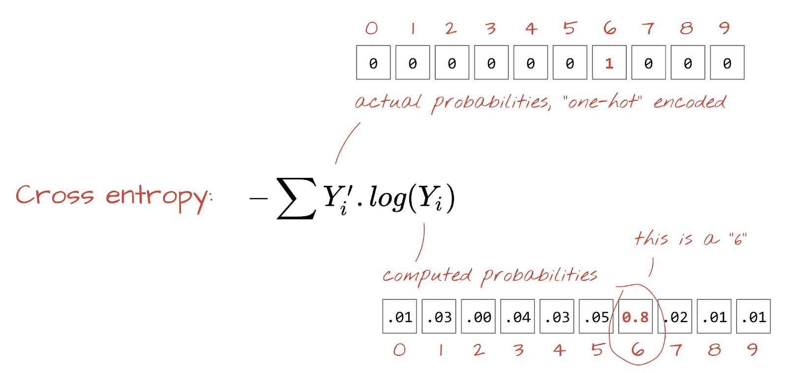
Cross-entropy loss
Now that our neural network produces predictions from input images, we need to measure how good they are, i.e. the distance between what the network tells us and the correct answers, often called "labels". Remember that we have correct labels for all the images in the dataset.
Any distance would work, but for classification problems the so-called "cross-entropy distance" is the most effective. We will call this our error or "loss" function:
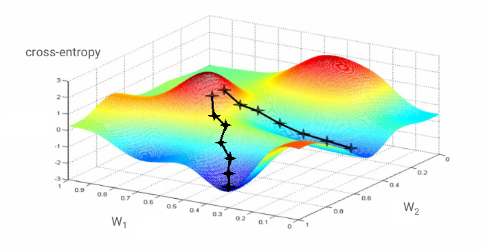
Gradient descent
"Training" the neural network actually means using training images and labels to adjust weights and biases so as to minimise the cross-entropy loss function. Here is how it works.
The cross-entropy is a function of weights, biases, pixels of the training image and its known class.
If we compute the partial derivatives of the cross-entropy relatively to all the weights and all the biases we obtain a "gradient", computed for a given image, label, and present value of weights and biases. Remember that we can have millions of weights and biases so computing the gradient sounds like a lot of work. Fortunately, TensorFlow does it for us. The mathematical property of a gradient is that it points "up". Since we want to go where the cross-entropy is low, we go in the opposite direction. We update weights and biases by a fraction of the gradient. We then do the same thing again and again using the next batches of training images and labels, in a training loop. Hopefully, this converges to a place where the cross-entropy is minimal although nothing guarantees that this minimum is unique.
Mini-batching and momentum
You can compute your gradient on just one example image and update the weights and biases immediately, but doing so on a batch of, for example, 128 images gives a gradient that better represents the constraints imposed by different example images and is therefore likely to converge towards the solution faster. The size of the mini-batch is an adjustable parameter.
This technique, sometimes called "stochastic gradient descent" has another, more pragmatic benefit: working with batches also means working with larger matrices and these are usually easier to optimise on GPUs and TPUs.
The convergence can still be a little chaotic though and it can even stop if the gradient vector is all zeros. Does that mean that we have found a minimum? Not always. A gradient component can be zero on a minimum or a maximum. With a gradient vector with millions of elements, if they are all zeros, the probability that every zero corresponds to a minimum and none of them to a maximum point is pretty small. In a space of many dimensions, saddle points are pretty common and we do not want to stop at them.
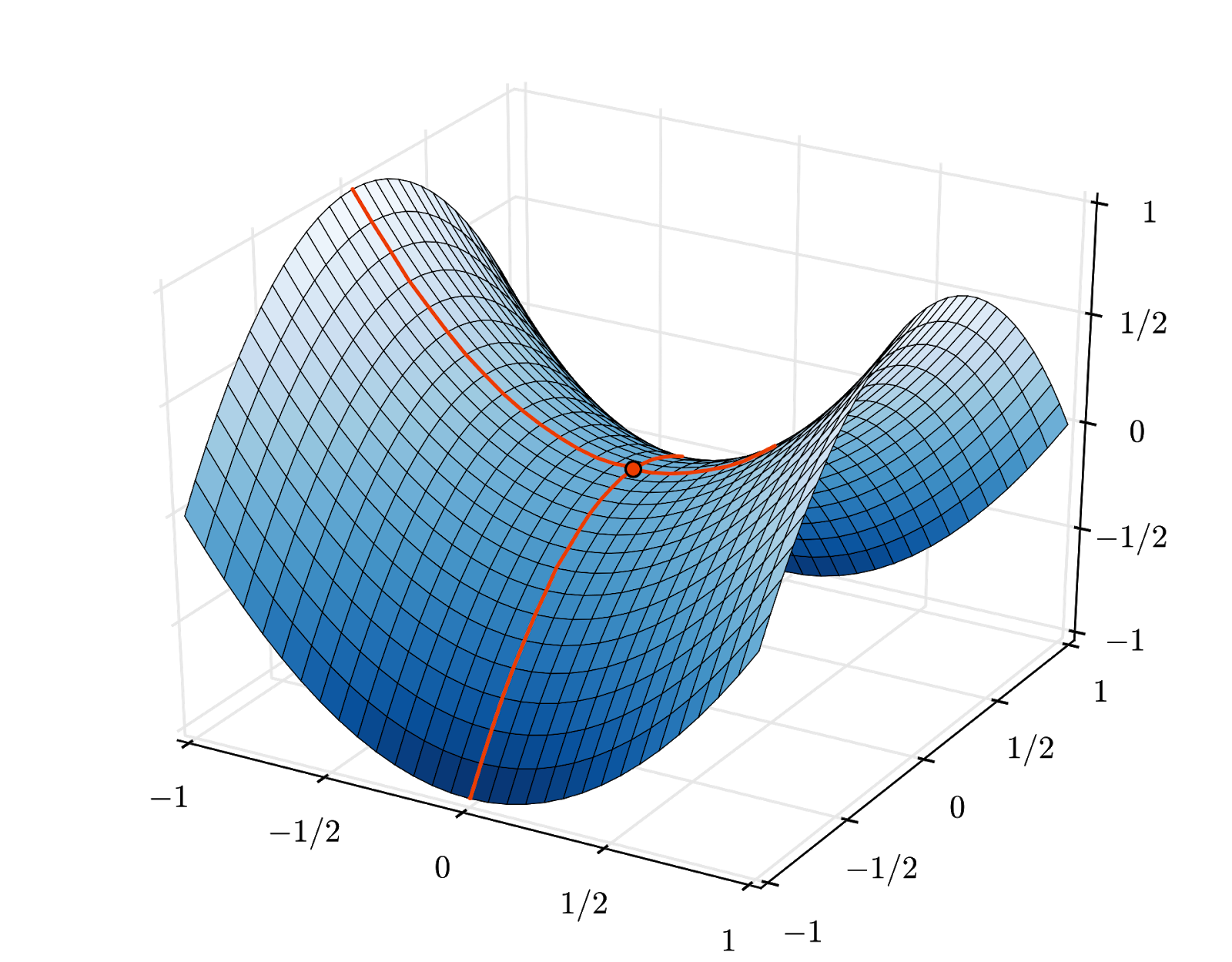
Illustration: a saddle point. The gradient is 0 but it is not a minimum in all directions. (Image attribution Wikimedia: By Nicoguaro - Own work, CC BY 3.0)
The solution is to add some momentum to the optimization algorithm so that it can sail past saddle points without stopping.
Glossary
batch or mini-batch: training is always performed on batches of training data and labels. Doing so helps the algorithm converge. The "batch" dimension is typically the first dimension of data tensors. For example a tensor of shape [100, 192, 192, 3] contains 100 images of 192x192 pixels with three values per pixel (RGB).
cross-entropy loss: a special loss function often used in classifiers.
dense layer: a layer of neurons where each neuron is connected to all the neurons in the previous layer.
features: the inputs of a neural network are sometimes called "features". The art of figuring out which parts of a dataset (or combinations of parts) to feed into a neural network to get good predictions is called "feature engineering".
labels: another name for "classes" or correct answers in a supervised classification problem
learning rate: fraction of the gradient by which weights and biases are updated at each iteration of the training loop.
logits: the outputs of a layer of neurons before the activation function is applied are called "logits". The term comes from the "logistic function" a.k.a. the "sigmoid function" which used to be the most popular activation function. "Neuron outputs before logistic function" was shortened to "logits".
loss: the error function comparing neural network outputs to the correct answers
neuron: computes the weighted sum of its inputs, adds a bias and feeds the result through an activation function.
one-hot encoding: class 3 out of 5 is encoded as a vector of 5 elements, all zeros except the 3rd one which is 1.
relu: rectified linear unit. A popular activation function for neurons.
sigmoid: another activation function that used to be popular and is still useful in special cases.
softmax: a special activation function that acts on a vector, increases the difference between the largest component and all others, and also normalizes the vector to have a sum of 1 so that it can be interpreted as a vector of probabilities. Used as the last step in classifiers.
tensor: A "tensor" is like a matrix but with an arbitrary number of dimensions. A 1-dimensional tensor is a vector. A 2-dimensions tensor is a matrix. And then you can have tensors with 3, 4, 5 or more dimensions.
5. Let's jump into the code
Back to the study notebook and this time, let's read the code.
Let's go through all the cell in this notebook.
Cell "Parameters"
The batch size, number of training epochs and location of the data files is defined here. Data files are hosted in a Google Cloud Storage (GCS) bucket which is why their address starts with gs://
Cell "Imports"
All the necessary Python libraries are imported here, including TensorFlow and also matplotlib for visualizations.
Cell "visualization utilities [RUN ME]****"
This cell contains uninteresting visualization code. It is collapsed by default but you can open it and look at the code when you have the time by double-clicking on it.
Cell "tf.data.Dataset: parse files and prepare training and validation datasets"
This cell used the tf.data.Dataset API to load the MNIST dataset form the data files. It is not necessary to spend too much time on this cell. If you are interested in the tf.data.Dataset API, here is a tutorial that explains it: TPU-speed data pipelines. For now, the basics are:
Images and labels (correct answers) from the MNIST dataset are stored in fixed length records in 4 files. The files can be loaded with the dedicated fixed record function:
imagedataset = tf.data.FixedLengthRecordDataset(image_filename, 28*28, header_bytes=16)
We now have a dataset of image bytes. They need to be decoded into images. We define a function for doing so. The image is not compressed so the function does not need to decode anything (decode_raw does basically nothing). The image is then converted to floating point values between 0 and 1. We could reshape it here as a 2D image but actually we keep it as a flat array of pixels of size 28*28 because that is what our initial dense layer expects.
def read_image(tf_bytestring):
    image = tf.io.decode_raw(tf_bytestring, tf.uint8)
    image = tf.cast(image, tf.float32)/256.0
    image = tf.reshape(image, [28*28])
    return image
We apply this function to the dataset using .map and obtain a dataset of images:
imagedataset = imagedataset.map(read_image, num_parallel_calls=16)
We do the same kind of reading and decoding for labels and we .zip images and labels together:
dataset = tf.data.Dataset.zip((imagedataset, labelsdataset))
We now have a dataset of pairs (image, label). This is what our model expects. We are not quite ready to use it in the training function yet:
dataset = dataset.cache()
dataset = dataset.shuffle(5000, reshuffle_each_iteration=True)
dataset = dataset.repeat()
dataset = dataset.batch(batch_size)
dataset = dataset.prefetch(tf.data.experimental.AUTOTUNE)
The tf.data.Dataset API has all the necessary utility function for preparing datasets:
.cache caches the dataset in RAM. This is a tiny dataset so it will work. .shuffle shuffles it with a buffer of 5000 elements. It is important that training data are well shuffled. .repeat loops the dataset. We will be training on it multiple times (multiple epochs). .batch pulls multiple images and labels together into a mini-batch. Finally, .prefetch can use the CPU to prepare the next batch while the current batch is being trained on the GPU.
The validation dataset is prepared in a similar way. We are now ready to define a model and use this dataset to train it.
Cell "Keras Model"
All of our models will be straight sequences of layers so we can use the tf.keras.Sequential style to create them. Initially here, it's a single dense layer. It has 10 neurons because we are classifying handwritten digits into 10 classes. It uses "softmax" activation because it is the last layer in a classifier.
A Keras model also needs to know the shape of its inputs. tf.keras.layers.Input can be used to define it. Here, input vectors are flat vectors of pixel values of length 28*28.
model = tf.keras.Sequential(
  [
    tf.keras.layers.Input(shape=(28*28,)),
    tf.keras.layers.Dense(10, activation='softmax')
  ])

model.compile(optimizer='sgd',
              loss='categorical_crossentropy',
              metrics=['accuracy'])

# print model layers
model.summary()

# utility callback that displays training curves
plot_training = PlotTraining(sample_rate=10, zoom=1)
Configuring the model is done in Keras using the model.compile function. Here we use the basic optimizer 'sgd' (Stochastic Gradient Descent). A classification model requires a cross-entropy loss function, called 'categorical_crossentropy' in Keras. Finally, we ask the model to compute the 'accuracy' metric, which is the percentage of correctly classified images.
Keras offers the very nice model.summary() utility that prints the details of the model you have created. Your kind instructor has added the PlotTraining utility (defined in the "visualization utilities" cell) which will display various training curves during the training.
Cell "Train and validate the model"
This is where the training happens, by calling model.fit and passing in both the training and validation datasets. By default, Keras runs a round of validation at the end of each epoch.
model.fit(training_dataset, steps_per_epoch=steps_per_epoch, epochs=EPOCHS,
          validation_data=validation_dataset, validation_steps=1,
          callbacks=[plot_training])
In Keras, it is possible to add custom behaviors during training by using callbacks. That is how the dynamically updating training plot was implemented for this workshop.
Cell "Visualize predictions"
Once the model is trained, we can get predictions from it by calling model.predict():
probabilities = model.predict(font_digits, steps=1)
predicted_labels = np.argmax(probabilities, axis=1)
Here we have prepared a set of printed digits rendered from local fonts, as a test. Remember that the neural network returns a vector of 10 probabilities from its final "softmax". To get the label, we have to find out which probability is the highest. np.argmax from the numpy library does that.
To understand why the axis=1 parameter is needed, please remember that we have processed a batch of 128 images and therefore the model returns 128 vectors of probabilities. The shape of the output tensor is [128, 10]. We are computing the argmax across the 10 probabilities returned for each image, thus axis=1 (the first axis being 0).
This simple model already recognises 90% of the digits. Not bad, but you will now improve this significantly.
6. Adding layers

To improve the recognition accuracy we will add more layers to the neural network.
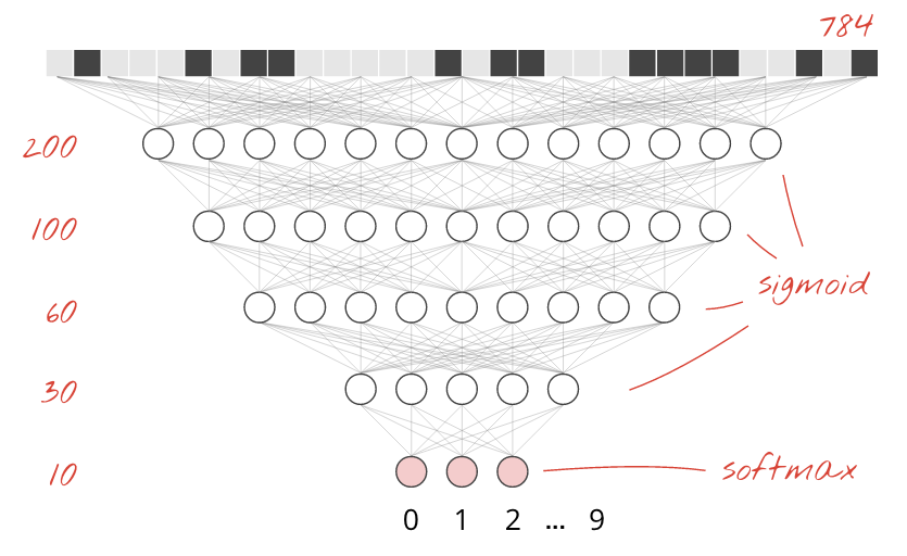
We keep softmax as the activation function on the last layer because that is what works best for classification. On intermediate layers however we will use the most classical activation function: the sigmoid:
For example, your model could look like this (do not forget the commas, tf.keras.Sequential takes a comma-separated list of layers):
model = tf.keras.Sequential(
  [
      tf.keras.layers.Input(shape=(28*28,)),
      tf.keras.layers.Dense(200, activation='sigmoid'),
      tf.keras.layers.Dense(60, activation='sigmoid'),
      tf.keras.layers.Dense(10, activation='softmax')
  ])
Look at the "summary" of you model. It now has at least 10 times more parameters. It should be 10x better! But for some reason, it isn't ...
The loss seems to have shot through the roof too. Something is not quite right.
7. Special care for deep networks
You have just experienced neural networks, as people used to design them in the 80's and 90's. No wonder they gave up on the idea, ushering the so-called "AI winter". Indeed, as you add layers, neural networks have more and more difficulties to converge.
It turns out that deep neural networks with many layers (20, 50, even 100 today) can work really well, provided a couple of mathematical dirty tricks to make them converge. The discovery of these simple tricks is one of the reasons for the renaissance of deep learning in the 2010's.
RELU activation

The sigmoid activation function is actually quite problematic in deep networks. It squashes all values between 0 and 1 and when you do so repeatedly, neuron outputs and their gradients can vanish entirely. It was mentioned for historical reasons, but modern networks use the RELU (Rectified Linear Unit) which looks like this:
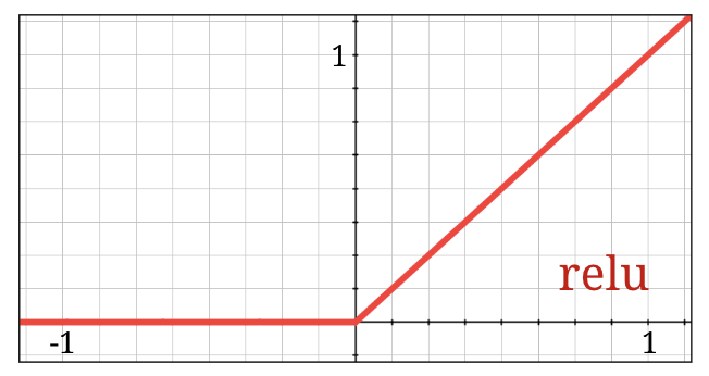
The relu on the other hand has a derivative of 1, at least on its right side. With RELU activation, even if the gradients coming from some neurons can be zero, there will always be others giving a clear non-zero gradient and training can continue at a good pace.
A better optimizer
In very high-dimensional spaces like here — we have on the order of 10K weights and biases — "saddle points" are frequent. These are points that are not local minima, but where the gradient is nevertheless zero and the gradient descent optimizer stays stuck there. TensorFlow has a full array of available optimizers, including some that work with an amount of inertia and will safely sail past saddle points.
Random initializations
The art of initializing weights biases before training is an area of research in itself, with numerous papers published on the topic. You can have a look at all the initializers available in Keras here. Fortunately, Keras does the right thing by default and uses the 'glorot_uniform' initializer which is the best in almost all cases.
There is nothing for you to do, since Keras already does the right thing.
NaN ???
The cross-entropy formula involves a logarithm and log(0) is Not a Number (NaN, a numerical crash if you prefer). Can the input to the cross-entropy be 0? The input comes from softmax which is essentially an exponential and an exponential is never zero. So we are safe!
Really? In the beautiful world of mathematics, we would be safe, but in the computer world, exp(-150), represented in float32 format, is as ZERO as it gets and the cross-entropy crashes.
Fortunately, there is nothing for you to do here either, since Keras takes care of this and computes softmax followed by the cross-entropy in an especially careful way to ensure numerical stability and avoid the dreaded NaNs.
Success?
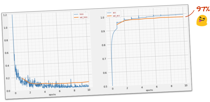
You should now be getting to 97% accuracy. The goal in this workshop is to get significantly above 99% so let's keep going.
If you are stuck, here is the solution at this point:
8. Learning rate decay
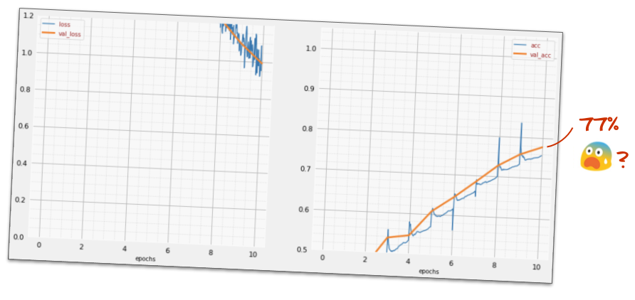
Maybe we can try to train faster? The default learning rate in the Adam optimizer is 0.001. Let's try to increase it.
Going faster does not seem to help a lot and what is all this noise?
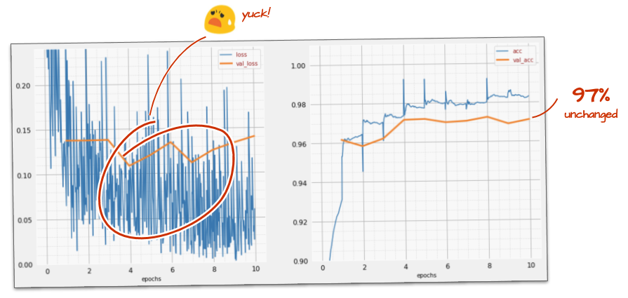
The training curves are really noisy and look at both validation curves: they are jumping up and down. This means that we are going too fast. We could go back to our previous speed, but there is a better way.

The good solution is to start fast and decay the learning rate exponentially. In Keras, you can do this with the tf.keras.callbacks.LearningRateScheduler callback.
Useful code for copy-pasting:
# lr decay function
def lr_decay(epoch):
  return 0.01 * math.pow(0.6, epoch)

# lr schedule callback
lr_decay_callback = tf.keras.callbacks.LearningRateScheduler(lr_decay, verbose=True)

# important to see what you are doing
plot_learning_rate(lr_decay, EPOCHS)
Do not forget to use the lr_decay_callback you have created. Add it to the list of callbacks in model.fit:
model.fit(..., callbacks=[plot_training, lr_decay_callback])
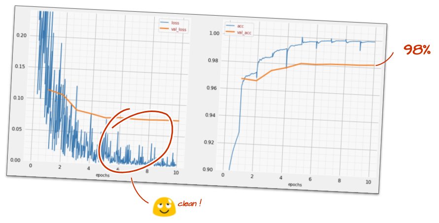
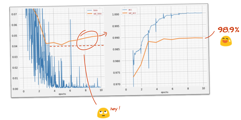
The impact of this little change is spectacular. You see that most of the noise is gone and the test accuracy is now above 98% in a sustained way.
9. Dropout, overfitting
The model seems to be converging nicely now. Let's try to go even deeper.
Does it help?
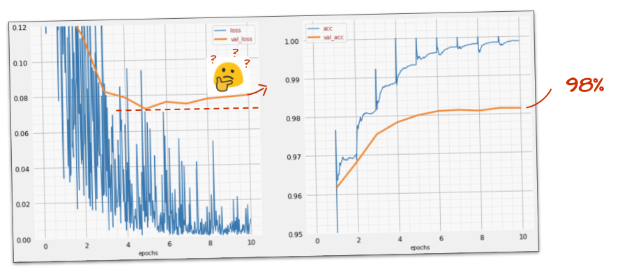
Not really, the accuracy is still stuck at 98% and look at the validation loss. It is going up! The learning algorithm works on training data only and optimises the training loss accordingly. It never sees validation data so it is not surprising that after a while its work no longer has an effect on the validation loss which stops dropping and sometimes even bounces back up.
This does not immediately affect the real-world recognition capabilities of your model, but it will prevent you from running many iterations and is generally a sign that the training is no longer having a positive effect.

This disconnect is usually called "overfitting" and when you see it, you can try to apply a regularisation technique called "dropout". The dropout technique shoots random neurons at each training iteration.
Did it work?
Noise reappears (unsurprisingly given how dropout works). The validation loss does not seem to be creeping up anymore, but it is higher overall than without dropout. And the validation accuracy went down a bit. This is a fairly disappointing result.
It looks like dropout was not the correct solution, or maybe "overfitting" is a more complex concept and some of its causes are not amenable to a "dropout" fix?
What is "overfitting"? Overfitting happens when a neural network learns "badly", in a way that works for the training examples but not so well on real-world data. There are regularisation techniques like dropout that can force it to learn in a better way but overfitting also has deeper roots.
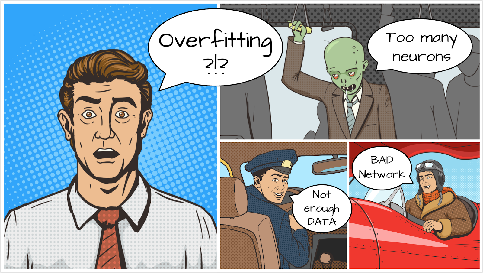
Basic overfitting happens when a neural network has too many degrees of freedom for the problem at hand. Imagine we have so many neurons that the network can store all of our training images in them and then recognise them by pattern matching. It would fail on real-world data completely. A neural network must be somewhat constrained so that it is forced to generalise what it learns during training.
If you have very little training data, even a small network can learn it by heart and you will see "overfitting". Generally speaking, you always need lots of data to train neural networks.
Finally, if you have done everything by the book, experimented with different sizes of network to make sure its degrees of freedom are constrained, applied dropout, and trained on lots of data you might still be stuck at a performance level that nothing seems to be able to improve. This means that your neural network, in its present shape, is not capable of extracting more information from your data, as in our case here.
Remember how we are using our images, flattened into a single vector? That was a really bad idea. Handwritten digits are made of shapes and we discarded the shape information when we flattened the pixels. However, there is a type of neural network that can take advantage of shape information: convolutional networks. Let us try them.
If you are stuck, here is the solution at this point:
10. [INFO] convolutional networks
In a nutshell
If all the terms in bold in the next paragraph are already known to you, you can move to the next exercise. If your are just starting out with convolutional neural networks, please read on.
Illustration: filtering an image with two successive filters made of 4x4x3=48 learnable weights each.
This is how a simple convolutional neural network looks in Keras:
model = tf.keras.Sequential([
    tf.keras.layers.Reshape(input_shape=(28*28,), target_shape=(28, 28, 1)),
    tf.keras.layers.Conv2D(kernel_size=3, filters=12, activation='relu'),
    tf.keras.layers.Conv2D(kernel_size=6, filters=24, strides=2, activation='relu'),
    tf.keras.layers.Conv2D(kernel_size=6, filters=32, strides=2, activation='relu'),
    tf.keras.layers.Flatten(),
    tf.keras.layers.Dense(10, activation='softmax')
])
In a layer of a convolutional network, one "neuron" does a weighted sum of the pixels just above it, across a small region of the image only. It adds a bias and feeds the sum through an activation function, just as a neuron in a regular dense layer would. This operation is then repeated across the entire image using the same weights. Remember that in dense layers, each neuron had its own weights. Here, a single "patch" of weights slides across the image in both directions (a "convolution"). The output has as many values as there are pixels in the image (some padding is necessary at the edges though). It is a filtering operation. In the illustration above, it uses a filter of 4x4x3=48 weights.
However, 48 weights will not be enough. To add more degrees of freedom, we repeat the same operation with a new set of weights. This produces a new set of filter outputs. Let's call it a "channel" of outputs by analogy with the R,G,B channels in the input image.
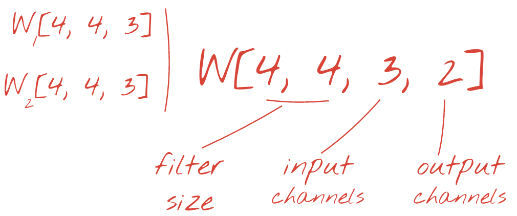
The two (or more) sets of weights can be summed up as one tensor by adding a new dimension. This gives us the generic shape of the weights tensor for a convolutional layer. Since the number of input and output channels are parameters, we can start stacking and chaining convolutional layers.
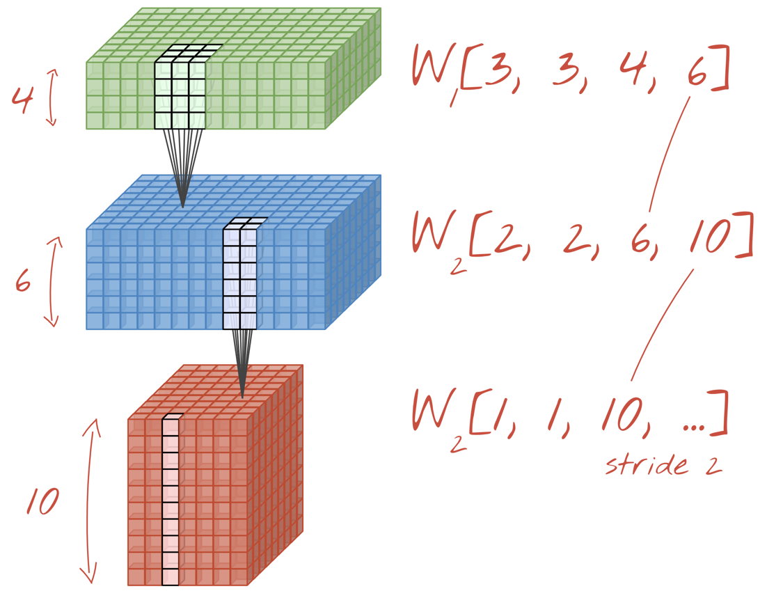
Illustration: a convolutional neural network transforms "cubes" of data into other "cubes" of data.
Strided convolutions, max pooling
By performing the convolutions with a stride of 2 or 3, we can also shrink the resulting data cube in its horizontal dimensions. There are two common ways of doing this:
- Strided convolution: a sliding filter as above but with a stride >1
- Max pooling: a sliding window applying the MAX operation (typically on 2x2 patches, repeated every 2 pixels)
Illustration: sliding the computing window by 3 pixels results in fewer output values. Strided convolutions or max pooling (max on a 2x2 window sliding by a stride of 2) are a way of shrinking the data cube in the horizontal dimensions.
The final layer
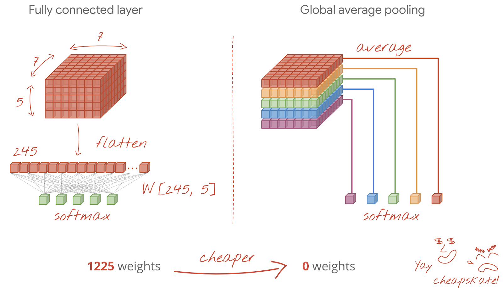
After the last convolutional layer, the data is in the form of a "cube". There are two ways of feeding it through the final dense layer.
The first one is to flatten the cube of data into a vector and then feed it to the softmax layer. Sometimes, you can even add a dense layer before the softmax layer. This tends to be expensive in terms of the number of weights. A dense layer at the end of a convolutional network can contain more than half the weights of the whole neural network.
Instead of using an expensive dense layer, we can also split the incoming data "cube" into as many parts as we have classes, average their values and feed these through a softmax activation function. This way of building the classification head costs 0 weights. In Keras, there is a layer for this: tf.keras.layers.GlobalAveragePooling2D().
Jump to the next section to build a convolutional network for the problem at hand.
11. A convolutional network
Let us build a convolutional network for handwritten digit recognition. We will use three convolutional layers at the top, our traditional softmax readout layer at the bottom and connect them with one fully-connected layer:
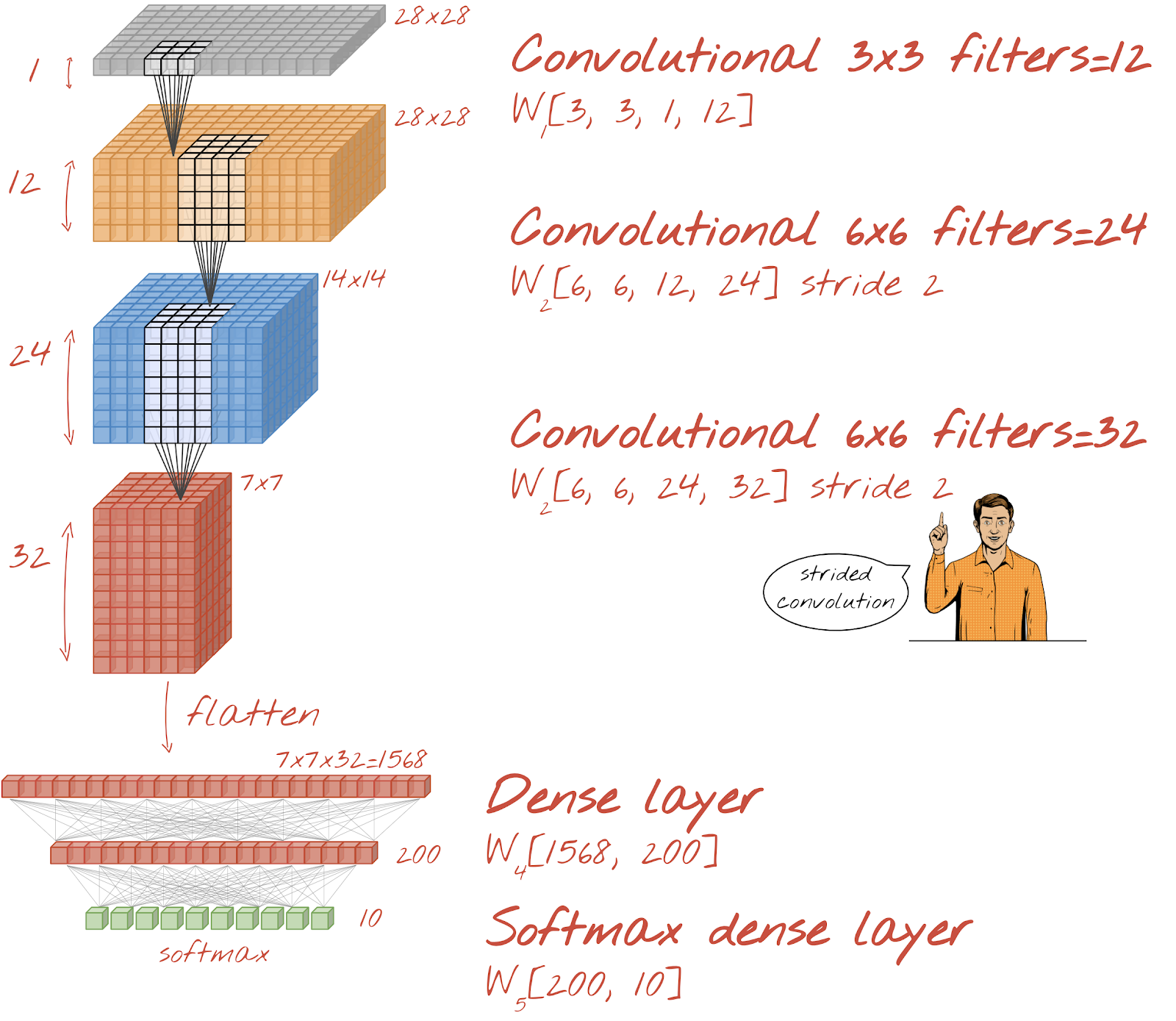
Notice that the second and third convolutional layers have a stride of two which explains why they bring the number of output values down from 28x28 to 14x14 and then 7x7.
Let's write the Keras code.
Special attention is needed before the first convolutional layer. Indeed, it expects a 3D ‘cube' of data but our dataset has so far been set up for dense layers and all the pixels of the images are flattened into a vector. We need to reshape them back into 28x28x1 images (1 channel for grayscale images):
tf.keras.layers.Reshape(input_shape=(28*28,), target_shape=(28, 28, 1))
You can use this line instead of the tf.keras.layers.Input layer you had up to now.
In Keras, the syntax for a ‘relu'-activated convolutional layer is:
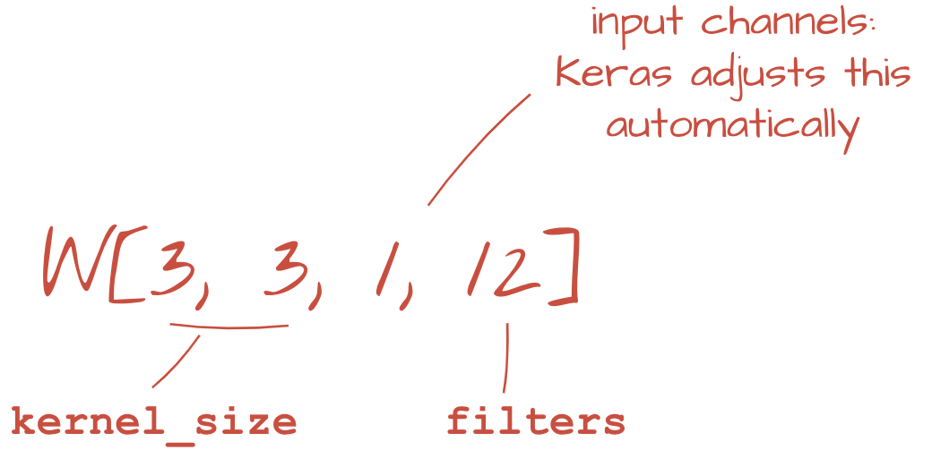
tf.keras.layers.Conv2D(kernel_size=3, filters=12, padding='same', activation='relu')
For a strided convolution, you would write:
tf.keras.layers.Conv2D(kernel_size=6, filters=24, padding='same', activation='relu', strides=2)
To flatten a cube of data into a vector so that it can be consumed by a dense layer:
tf.keras.layers.Flatten()
And for dense layer, the syntax has not changed:
tf.keras.layers.Dense(200, activation='relu')
Did your model break the 99% accuracy barrier? Pretty close... but look at the validation loss curve. Does this ring a bell?
Also look at the predictions. For the first time, you should see that most of the 10,000 test digits are now correctly recognized. Only about 4½ rows of misdetections remain (about 110 digits out of 10,000)
If you are stuck, here is the solution at this point:
12. Dropout again
The previous training exhibits clear signs of overfitting (and still falls short of 99% accuracy). Should we try dropout again?
How did it go this time?
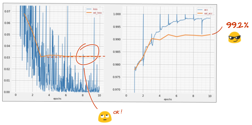
It looks like dropout has worked this time. The validation loss is not creeping up anymore and the final accuracy should be way above 99%. Congratulations!
The first time we tried to apply dropout, we thought we had an overfitting problem, when in fact the problem was in the architecture of the neural network. We could not go further without convolutional layers and there is nothing dropout could do about that.
This time, it does look like overfitting was the cause of the problem and dropout actually helped. Remember, there are many things that can cause a disconnect between the training and validation loss curves, with the validation loss creeping up. Overfitting (too many degrees of freedom, used badly by the network) is only one of them. If your dataset is too small or the architecture of your neural network is not adequate, you might see a similar behavior on the loss curves, but dropout will not help.
13. Batch normalization

Finally, let's try to add batch normalization.
That's the theory, in practice, just remember a couple of rules:
Let's play by the book for now and add a batch norm layer on each neural network layer but the last. Do not add it to the last "softmax" layer. It would not be useful there.
# Modify each layer: remove the activation from the layer itself.
# Set use_bias=False since batch norm will play the role of biases.
tf.keras.layers.Conv2D(..., use_bias=False),
# Batch norm goes between the layer and its activation.
# The scale factor can be turned off for Relu activation.
tf.keras.layers.BatchNormalization(scale=False, center=True),
# Finish with the activation.
tf.keras.layers.Activation('relu'),
How is the accuracy now?
With a little bit of tweaking (BATCH_SIZE=64, learning rate decay parameter 0.666, dropout rate on dense layer 0.3) and a bit of luck, you can get to 99.5%. The learning rate and dropout adjustments were done following the "best practices" for using batch norm:
- Batch norm helps neural networks converge and usually allows you to train faster.
- Batch norm is a regularizer. You can usually decrease the amount of dropout you use, or even not use dropout at all.
The solution notebook has a 99.5% training run:
14. Train in the cloud on powerful hardware: AI Platform

You will find a cloud-ready version of the code in the mlengine folder on GitHub, along with instructions for running it on Google Cloud AI Platform. Before you can run this part, you will have to create a Google Cloud account and enable billing. The resources necessary to complete the lab should be less than a couple of dollars (assuming 1h of training time on one GPU). To prepare your account:
- Create a Google Cloud Platform project ( http://cloud.google.com/console).
- Enable billing.
- Install the GCP command line tools ( GCP SDK here).
- Create a Google Cloud Storage bucket (put in the region
us-central1). It will be used to stage the training code and store your trained model. - Enable the necessary APIs and request the necessary quotas (run the training command once and you should get error messages telling you what to enable).
15. Congratulations!
You have built your first neural network and trained it all the way to 99% accuracy. The techniques learned along the way are not specific to the MNIST dataset, actually they are widely used when working with neural networks. As a parting gift, here is the "cliff's notes" card for the lab, in cartoon version. You can use it to remember what you have learned:

Next steps
- After fully-connected and convolutional networks, you should have a look at recurrent neural networks.
- To run your training or inference in the cloud on a distributed infrastructure, Google Cloud provides AI Platform.
- Finally, we love feedback. Please tell us if you see something amiss in this lab or if you think it should be improved. We handle feedback through GitHub issues [ feedback link].

|
|
 The author: Martin GörnerTwitter:
All cartoon images in this lab copyright: alexpokusay / 123RF stock photos