Lab 2: Data Analysis & Multimodal Insights

1. Introduction

In the previous lab, you aggregated fragmented shipping logs and traced the cargo transponder to New York. However, arrival records show the container was immediately re-routed to avoid customs detection. The trail has now led you to the Port of Rio de Janeiro, a sprawling port with thousands of containers. Finding the right container among thousands of others is a difficult task.

In this lab, you'll use BigQuery's built-in AI capabilities to "read" unstructured port security images and detect thermal anomalies in sensor data, all using standard SQL. You'll then export vector embeddings to AlloyDB and run a vector search to match a fragmented telemetry signal to the missing container.

What you'll do

• Scan port security images to identify the stolen container using BigQuery AI
• Detect a thermal anomaly using BigQuery AI to confirm the container was stolen, not misplaced
• Generate vector embeddings and load them into AlloyDB for real-time search
• Match a fragmented telemetry beacon signal to locate the stolen container using Vector Search
• Explore investigation data with natural language using Conversational Analytics

What you'll need

• A web browser such as Chrome
• A Google Cloud project with billing enabled
• Basic familiarity with SQL and Google Cloud Console

This codelab is for intermediate developers.

The resources created in this codelab should cost less than $5.

2. Before You Begin

Start Cloud Shell

You will use Google Cloud Shell to download the code, run setup scripts, and deploy the application.

1. In a new browser tab, open the Cloud Shell: shell.cloud.google.com
2. Once connected, set your project ID and confirm your environment:

gcloud config set project <<YOUR_PROJECT_ID>>
export PROJECT_ID=$(gcloud config get-value project)
export REGION=us-central1

You should see a message similar to:

Your active configuration is: [cloudshell-####]
Updated property [core/project]

Clone the Repository

Clone the codelab repository to your Cloud Shell environment:

cd ~/
git clone --filter=blob:none --no-checkout https://github.com/GoogleCloudPlatform/devrel-demos.git
cd ~/devrel-demos
git sparse-checkout init --cone
git sparse-checkout set codelabs/bigquery-alloydb-insights
git checkout main
cd codelabs/bigquery-alloydb-insights/

Enable APIs

Run this command in Cloud Shell to enable all required APIs for this lab:

gcloud services enable \
  aiplatform.googleapis.com \
  bigquery.googleapis.com \
  bigqueryconnection.googleapis.com \
  alloydb.googleapis.com

On successful execution, you should see a message similar to:

Operation "operations/..." finished successfully.

3. Set Up Your Environment

Before you can analyze images and telemetry data, you need to set up the infrastructure for this lab. You'll run two scripts: one kicks off AlloyDB provisioning in the background, and the other creates all the BigQuery resources you'll need.

Step 1: Start AlloyDB Deployment (Background)

AlloyDB cluster provisioning takes ~10 minutes, so you'll kick it off first and let it run in the background while you work through the BigQuery sections. The script will automatically record your active project settings to a local .env file so that your configuration is saved even if your Cloud Shell terminal closes or restarts.

chmod +x scripts/setup_alloydb.sh
nohup ./scripts/setup_alloydb.sh > /dev/null 2>&1 &
echo "AlloyDB deployment started in background (PID: $!)"

Step 2: Run the Setup Script

This script creates the BigQuery dataset, Cloud Resource connection, IAM grants, GCS bucket, and loads all the sensor data you'll analyze in this lab. It will also read and verify the environment variables saved in the .env file.

chmod +x scripts/setup_lab.sh
./scripts/setup_lab.sh

The script takes about a minute to run. When it finishes, you'll see a summary of everything it created.

📝 Note on environment resets If your Cloud Shell session times out or restarts at any point during this lab, you can restore your terminal variables immediately by running:

source scripts/setenv.sh

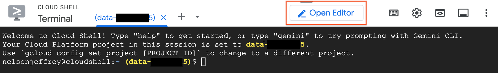
Step 3: Launch Cloud Shell Editor

You've been using the Cloud Shell terminal so far. Now switch to the full Cloud Shell Editor, which gives you a VS Code-like workspace with integrated BigQuery support.

1. In the Cloud Shell terminal pane at the bottom of your screen, click the Open Editor button to launch the Cloud Shell Editor workspace.

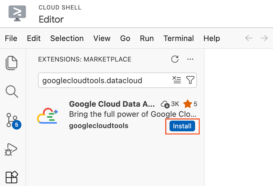
Step 4: Install the Data Agent Kit Extension

The Google Cloud Data Agent Kit extension provides deep integration with Google Cloud data services directly within your editor, allowing you to interact with BigQuery, AlloyDB, Cloud Storage, and more without switching contexts.

1. In the Cloud Shell Editor, click the Extensions icon in the Activity Bar on the far left side of the screen (it looks like four squares).
2. In the search bar at the top of the Extensions pane, type googlecloudtools.datacloud.
3. Locate the extension named Google Cloud Data Agent Kit published by Google Cloud.
4. Click the Install button.
5. A prompt will appear asking, "Do you trust publisher ‘googlecloudtools' and their extensions?". Click Trust Publishers & Install to proceed.

Step 5: Authenticate and Configure the Extension

After installation, connect the extension to your Google Cloud project.

1. An onboarding page titled "Google Cloud Data Agent Kit Onboarding" should automatically open. Click Sign in to Google Cloud. Follow any browser prompts to allow access.
2. A "Setup in progress" modal will appear. The extension will automatically check for required dependencies like the Google Cloud CLI.
3. In the Configuration Summary section, locate the project field. Click the dropdown and select your Google Cloud project. Set your region as us-central1.
4. Wait for the setup checks to finish. Once you see "Setup Complete!", click Configure MCP Servers.

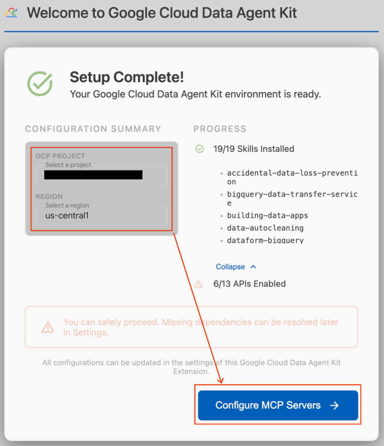
5. Select BigQuery and AlloyDB under MCP Configuration and then click Get Started.

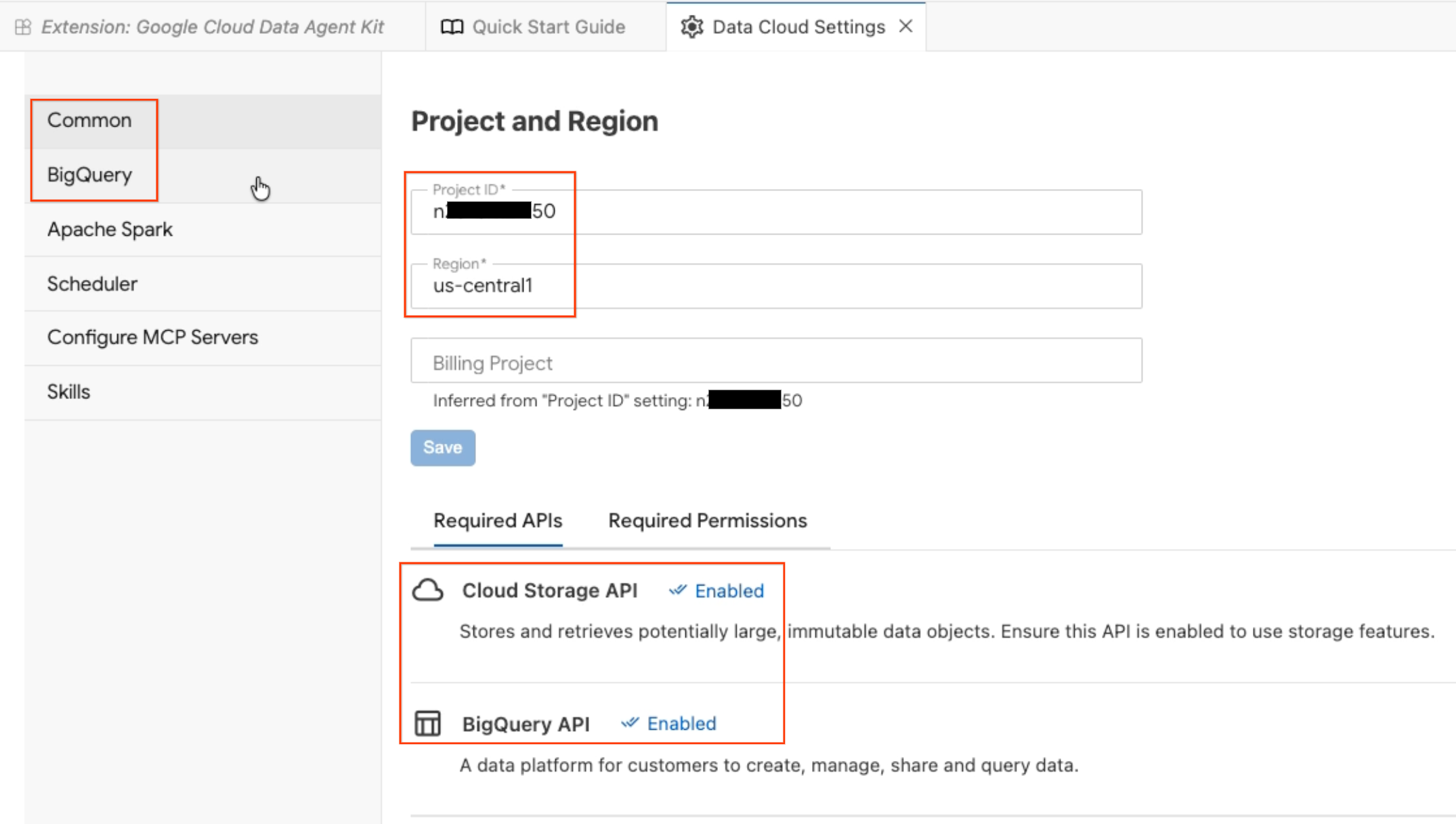
Step 6: Explore Configuration Options

Once setup is complete, you'll land on the "Get started with Google Cloud Data Agent Kit" dashboard.

1. Under "Setup & Configuration", click Get Started.
2. This opens the Data Agent Configuration panel. Explore the tabs:
   • Project and Region: Verify your selected Project ID and check that the required APIs (Cloud Storage API, BigQuery API, Catalog API, and AlloyDB API) are enabled.
   • BigQuery: Configure the default location for your BigQuery queries. Use the region us-central1.
   • Configure MCP Servers: View the enabled MCP servers (BigQuery, Notebooks, AlloyDB, etc.) that allow AI agents to securely interact with your data.
   • Skills: Explore pre-built skills that provide agents with specialized capabilities for complex data tasks.

Step 7: Verify with BigQuery

Confirm that everything is working by running a quick query against a public dataset.

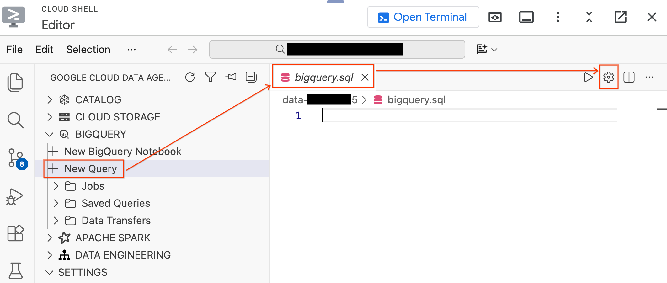
1. In the Data Agent Kit pane on the left, expand the BigQuery section and click New Query to open a new query editor tab.
2. Save the file by pressing Ctrl+S (Windows/Linux) or Cmd+S (macOS) and name it bigquery. This tab will be used for all of your BigQuery operations.
3. Click Query Settings with the bigquery.sql tab active, select BigQuery as the Data Source, and click Save.

Tab-Specific Settings: The Data Agent Kit extension saves connection configurations per tab. This means you can keep bigquery.sql open alongside other SQL tabs, and switching between them will automatically toggle the active database connection.

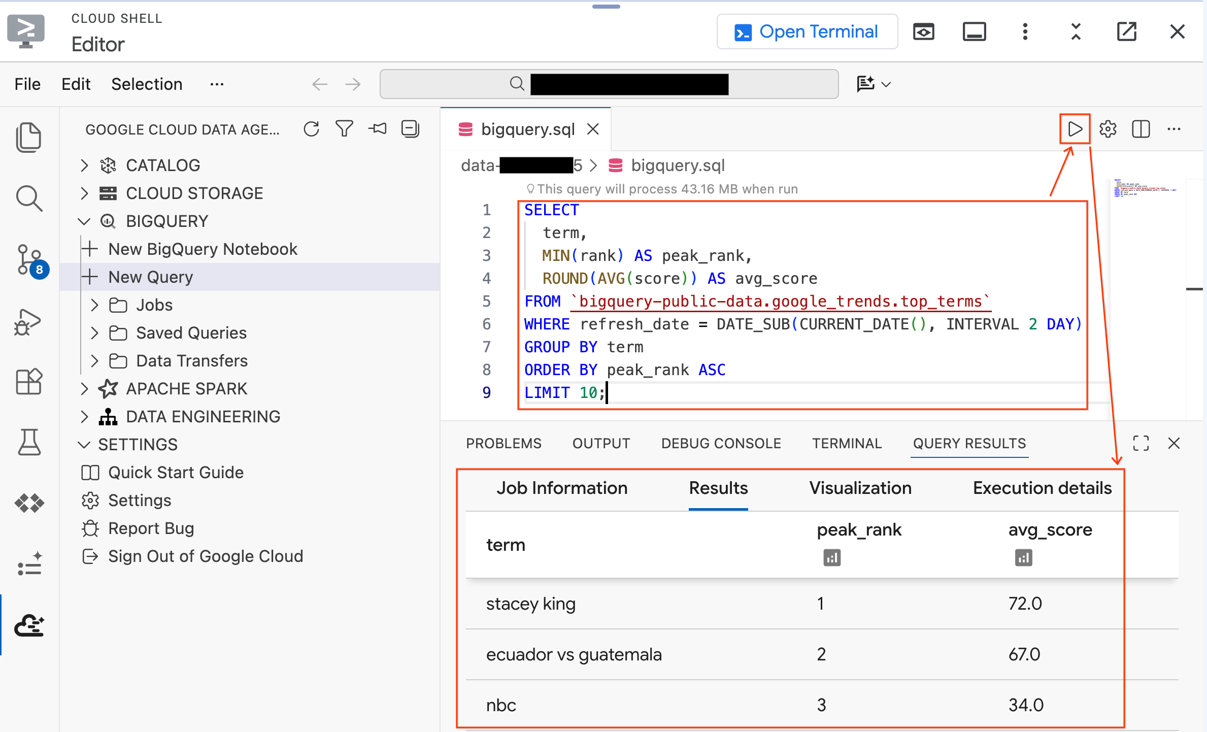
3. Run the following query against a public dataset:

SELECT
  term,
  MIN(rank) AS peak_rank,
  ROUND(AVG(score)) AS avg_score
FROM `bigquery-public-data.google_trends.top_terms`
WHERE refresh_date = DATE_SUB(CURRENT_DATE(), INTERVAL 2 DAY)
GROUP BY term
ORDER BY peak_rank ASC
LIMIT 10;

4. You should see the top 10 trending Google search terms from the past few days. If results appear, your extension is connected and ready.

Now try a query against the lab data your setup script just created. Replace the existing query with this one:

SELECT * FROM `lost_cargo_dataset.telemetry_data` LIMIT 5;

You should see telemetry log entries with shipment_id and telemetry_string columns. This is the data you'll be analyzing throughout the lab.

Running queries. Throughout this lab, you'll paste SQL into your .sql editor tab. If you highlight a specific statement and click Run Query, only that statement executes. If nothing is highlighted, clicking Run executes everything in the file. A simple workflow: each time you reach a new query step, replace the previous contents with the new SQL so the file only contains the query you want to run.

Section Recap: You kicked off the AlloyDB deployment in the background, ran the setup script, and configured the Cloud Shell Editor with the Data Agent Kit extension.

4. Scanning the Security Footage

The investigation team has recovered security footage from the Port of Rio de Janeiro showing rows of shipping containers. From Lab 1, you know the target container is red. Now you need to identify exactly which red container it is.

You'll create an Object Table that lets BigQuery "see" the security images in Cloud Storage, then use the AI.GENERATE function to prompt Gemini to extract structured data from each image.

Stay in the Editor! Be sure to continue running all SQL queries in this lab directly inside your Cloud Shell Editor workspace using the Data Agent Kit extension.

Step 1: Create the Object Table

An Object Table is a special BigQuery table that acts as an index over unstructured files (images, PDFs, audio) stored in Cloud Storage. It doesn't copy the files into BigQuery; it creates a queryable reference so AI functions can "see" them.

In your bigquery.sql tab in the editor, run the following statement to create the Object Table pointing to the port security images in your project's bucket:

SET @@location = 'us-central1';

EXECUTE IMMEDIATE CONCAT("""
  CREATE OR REPLACE EXTERNAL TABLE `lost_cargo_dataset.port_security_images`
  WITH CONNECTION `us-central1.lost_cargo_conn`
  OPTIONS (
    object_metadata = 'SIMPLE',
    uris = ['gs://""", @@project_id, """-lab2/images/*']
  );
""");

Take a quick look at what BigQuery can now see:

SELECT uri, content_type FROM `lost_cargo_dataset.port_security_images` LIMIT 5;

Each row represents one image file in Cloud Storage. BigQuery can now pass these images directly to AI models.

Step 2: Analyze the Security Images

Now use BigQuery's AI.GENERATE function to analyze each security image. This single SQL query prompts Gemini to examine every image and return structured data:

SELECT
  uri,
  AI.GENERATE(
    (
      'Examine this port security image. Identify any shipping container IDs visible on the container and provide a one-word color of the container.',
      ref
    ),
    output_schema => 'detected_container_id STRING, color STRING'
  ).* EXCEPT (full_response, status)
FROM `lost_cargo_dataset.port_security_images`;

Structured Output in SQL: Notice the output_schema => 'detected_container_id STRING, color STRING' parameter. This tells the Gemini model to return structured JSON that BigQuery natively casts into typed columns, meaning no post-processing is needed.

Step 3: Identify the Target Container

Examine the results. Look for the row where the color column shows "Red" (or some red variation). Note down the detected_container_id. This is your target: MV-CAPYBARA-003.

🔍 Container Clue Unlocked: The Gemini model successfully analyzed the security image and extracted the container's metadata. You have unlocked the target ID: MV-CAPYBARA-003. Keep this ID handy as we search for its route!

Step 4: Verify the Visual Match

To see the actual image that was analyzed without leaving your editor:

1. Click Cloud Storage in the Data Agent Kit pane on the left.
2. Expand your bucket (YOUR_PROJECT_ID-lab2/images/) and click on the image file corresponding to the red container to view it directly in the editor.

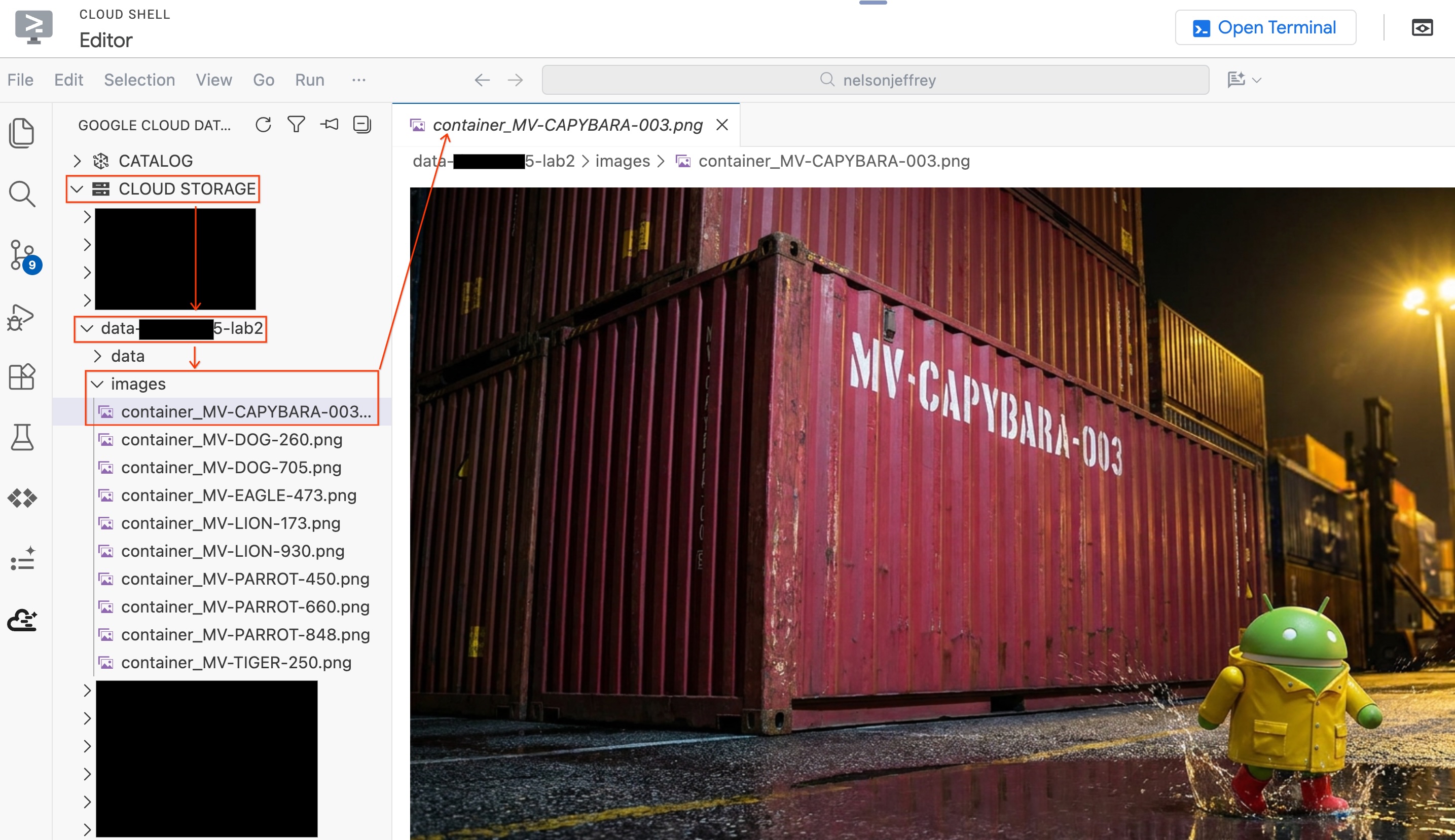
Section Recap: You created an Object Table to give BigQuery access to port security images, then used AI.GENERATE to extract structured container data from each image. The Red container has been identified as MV-CAPYBARA-003.

5. Confirming the Theft

You've identified the missing container as MV-CAPYBARA-003, but was it stolen or simply misplaced? Manifest logs indicate this specific container was parked adjacent to environmental sensor SENS-99. If the thieves deliberately disabled the container's onboard refrigeration unit before moving it, SENS-99 might have recorded a sudden thermal exhaust spike.

Let's use anomaly detection to prove the container was tampered with.

1. First, explore the historical baseline. These are the normal readings from SENS-99 over the past several hours:

SELECT * FROM `lost_cargo_dataset.thermal_history`
ORDER BY reading_time DESC
LIMIT 50;

Notice the temperatures hover in a tight range around 75-78°F. This is what normal looks like.

2. Now look at the current batch of readings from the same sensor:

SELECT * FROM `lost_cargo_dataset.thermal_current`
ORDER BY thermal_reading DESC
LIMIT 50;

See that 148.4°F reading near the top? Everything else looks normal. That spike would indicate either a refrigeration unit failure or deliberate tampering. Let's find out.

3. Run the anomaly detection. BigQuery's AI.DETECT_ANOMALIES uses the pre-trained TimesFM foundation model to analyze time-series patterns and flag outliers automatically, with zero model training required:

SELECT *
FROM AI.DETECT_ANOMALIES(
  TABLE `lost_cargo_dataset.thermal_history`,
  TABLE `lost_cargo_dataset.thermal_current`,
  data_col => 'thermal_reading',
  timestamp_col => 'reading_time',
  id_cols => ['sensor_id']
)
WHERE is_anomaly = TRUE;

4. Examine the results. The 148.4°F reading should be flagged as an anomaly with a high anomaly probability, confirming that something unusual happened near the container area.

🔍 Tampering Clue Unlocked: The TimesFM model flagged the 148.4°F temperature spike as a highly anomalous reading, confirming that the container's refrigeration unit was disabled. Keep this indicator of active tampering in mind as we set up our search backend!

Section Recap: You used BigQuery's AI.DETECT_ANOMALIES function to leverage the pre-trained TimesFM model. By running a single SQL query, you automatically identified outliers and isolated the anomalous tampering event without writing any complex machine learning code or training models from scratch.

6. Preparing the Tracking System

The container has been confirmed stolen and is no longer in Rio de Janeiro. Each container in the fleet broadcasts telemetry beacon signals: sensor readings, GPS fragments, and status logs. If the stolen container's beacon is still transmitting, you can match it against known signatures to find it.

BigQuery excels at the analytical work you've done so far, but locating a container in real time requires low-latency operational queries. AlloyDB, a fully managed PostgreSQL-compatible database, is built for exactly this: vector search queries fast enough for a live tracking system. You'll load your telemetry embeddings into AlloyDB and use it to match the beacon signal.

The AlloyDB cluster you kicked off in the background earlier should be ready by now. Let's configure it directly from your editor.

Step 1: Connect to AlloyDB from the Editor

Instead of switching to the Cloud Console, you can connect to AlloyDB directly using the Data Agent Kit extension.

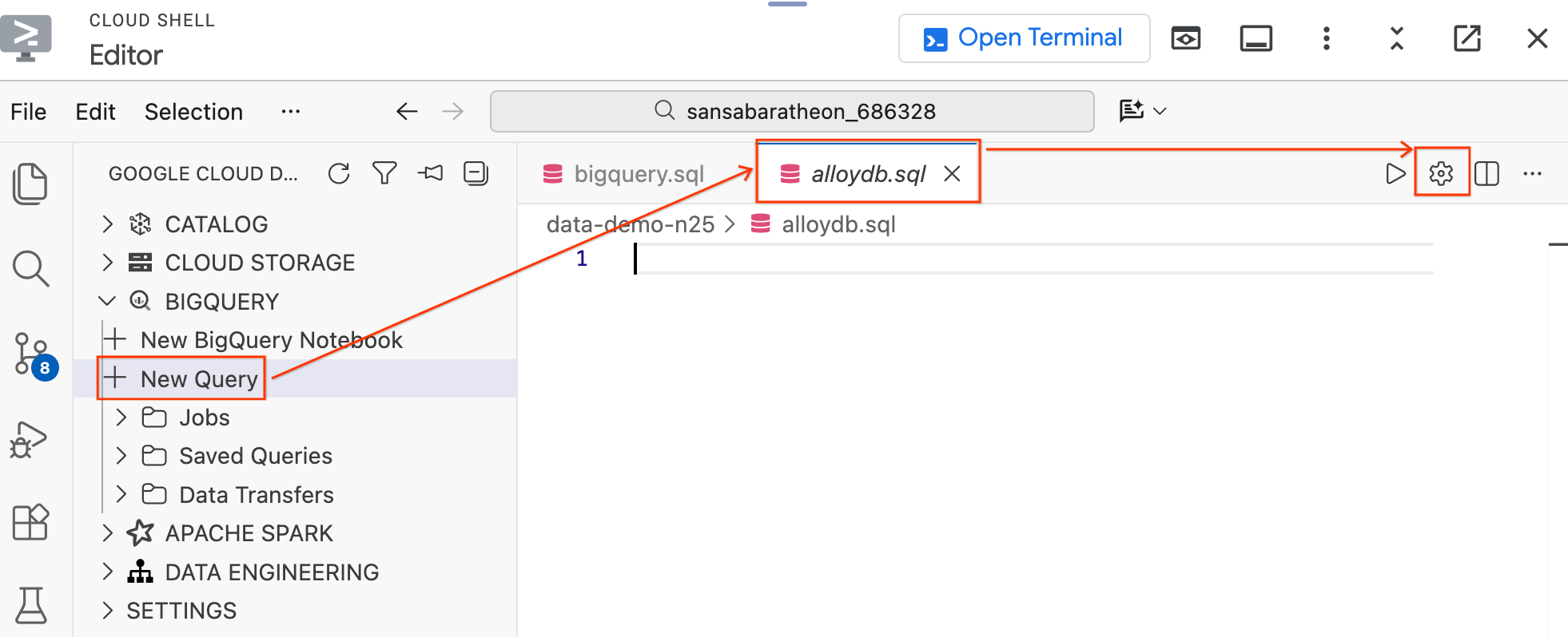
1. In the Data Agent Kit pane on the left under the BigQuery section, click New Query to open a new query editor tab.
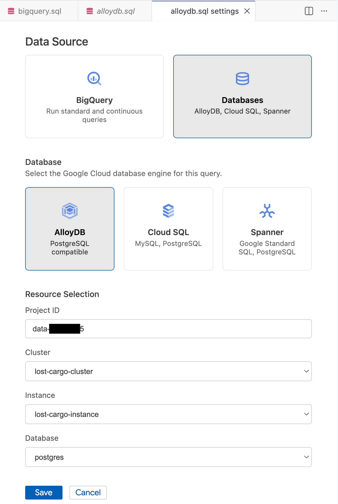
2. Save the file by pressing Ctrl+S (Windows/Linux) or Cmd+S (macOS) and name it alloydb. This tab will be used for all AlloyDB queries.
3. Click the gear icon to open the Query Settings modal.

4. In the Query Settings modal, under Data Source, select Databases.
5. Under Database, select AlloyDB.
6. Fill in the Resource Selection details:
   • Project ID: Enter your Google Cloud Project ID.
   • Cluster: Select lost-cargo-cluster.
   • Instance: Select lost-cargo-instance.
   • Database: Select postgres.
7. Click Save.

Developer Tip: You now have two query tabs open: bigquery.sql (for BigQuery queries) and alloydb.sql (for AlloyDB queries). Each tab retains its own data source configuration, allowing you to switch between them easily.

Step 2: Enable the Vector Extension and Create the Table

Now that you are connected to AlloyDB, you need to enable the necessary AI extensions and create the table that will receive the embedded telemetry data.

1. In your active .sql tab, paste the following commands to enable the required extensions:

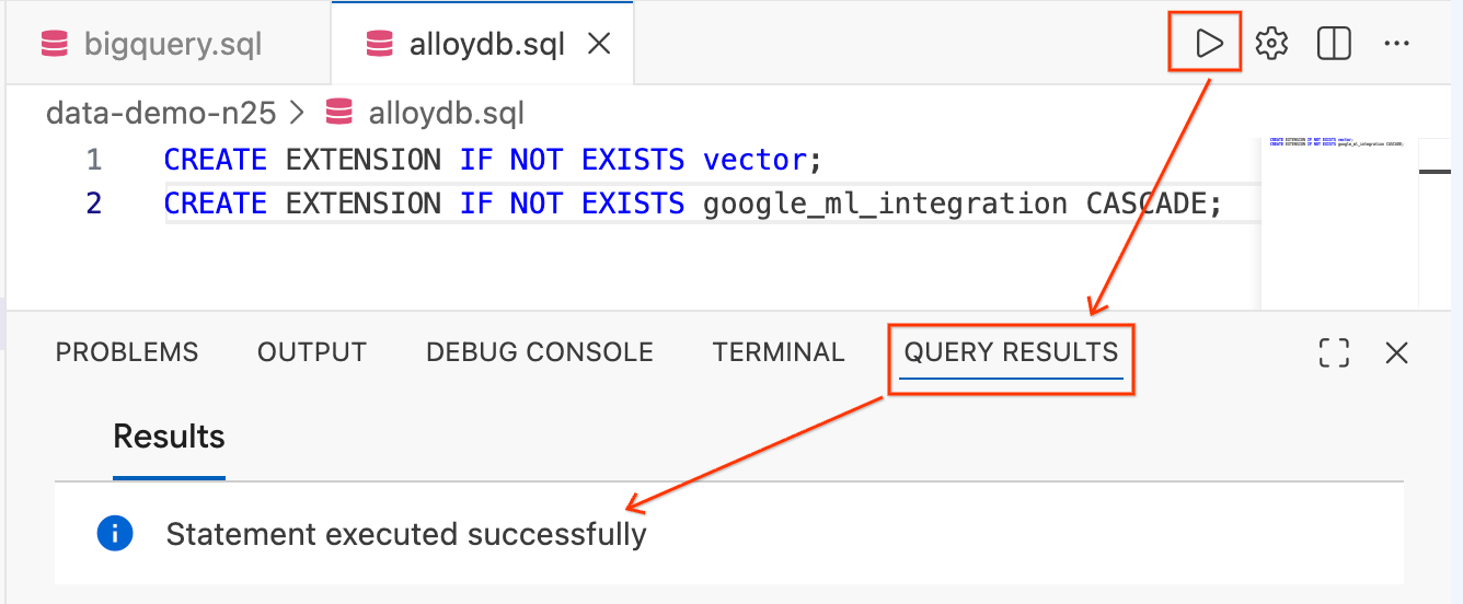
CREATE EXTENSION IF NOT EXISTS vector;
CREATE EXTENSION IF NOT EXISTS google_ml_integration CASCADE;

2. Highlight the text and click the Run Query button (the play icon) in the top right of the editor.
3. Check the Query Results terminal panel at the bottom of your screen. It should say Statement executed successfully.

4. Next, replace the text in your editor with the following statement to create the telemetry table:

CREATE TABLE IF NOT EXISTS vessel_telemetry (
    entry_id SERIAL PRIMARY KEY,
    shipment_id VARCHAR(50),
    telemetry_string TEXT,
    embedding_vector vector(768)
);

5. Run this query just like the last one. Confirm it executes successfully in the bottom panel.

The vector(768) type comes from the pgvector extension you just enabled. The 768 dimensions match the output of Google's text-embedding-005 model, which you'll use in BigQuery to generate the embeddings.

Section Recap: You connected to AlloyDB directly from your Cloud Shell Editor, enabled the pgvector and google_ml_integration extensions, and created the target table. AlloyDB is now ready to serve as the operational backend for real-time telemetry matching.

7. Building the Search Index

Now you need to get the telemetry data into AlloyDB so it can power real-time beacon matching. Raw telemetry logs are messy and variable-length, which isn't ideal for similarity search. You'll use BigQuery's AI functions to summarize each log with Gemini and convert each summary into a 768-dimensional vector embedding. Then you'll export the enriched data to Cloud Storage and import it into AlloyDB.

What is reverse ETL? Traditional ETL moves raw data into a data warehouse for analysis. Reverse ETL does the opposite: it pushes processed, enriched data out of the warehouse and into operational systems. Here, BigQuery generates the embeddings (analytics workload), then you export them to Cloud Storage and import them into AlloyDB (operational workload for low-latency vector search).

Step 1: Generate Embeddings in BigQuery

Switch your editor tab back to bigquery.sql (which remains connected to BigQuery).

Now, run the following query to summarize each telemetry log with Gemini and generate vector embeddings:

CREATE OR REPLACE TABLE `lost_cargo_dataset.telemetry_embeddings_export` AS
WITH summarized_telemetry AS (
  SELECT
    shipment_id,
    telemetry_string,
    AI.GENERATE(
      CONCAT('Summarize this telemetry log for vector search: ', telemetry_string)
    ).result AS summary
  FROM `lost_cargo_dataset.telemetry_data`
),
telemetry_embeddings AS (
  SELECT
    shipment_id,
    telemetry_string,
    AI.EMBED(summary, endpoint => 'text-embedding-005').result AS embedding
  FROM summarized_telemetry
)
SELECT
  shipment_id,
  telemetry_string,
  TO_JSON_STRING(embedding) AS embedding_vector
FROM telemetry_embeddings;

What is AI.EMBED? The AI.EMBED function converts text into a high-dimensional vector embedding. Semantically similar texts produce vectors that are mathematically close together.

Semantic Similarity: Keyword search looks for exact matches (e.g., "cooling" only matches "cooling"). Semantic similarity understands the meaning behind the words. For example, "Cooling unit offline" and "Refrigeration system malfunction" share zero identical words but represent the exact same concept. This allows us to match our fragmented beacon signal to the stored telemetry log even if they use different phrasing.

Step 2: Preview the Enriched Data

Before exporting, take a look at what you've created. This query shows the shipment IDs and the first 80 characters of each summary and embedding:

SELECT
  shipment_id,
  SUBSTR(telemetry_string, 1, 80) AS telemetry_preview,
  SUBSTR(embedding_vector, 1, 80) AS embedding_preview
FROM `lost_cargo_dataset.telemetry_embeddings_export`
LIMIT 5;

Each row now contains a shipment ID, the original telemetry log, and a 768-dimensional embedding vector. This is the data you'll push into AlloyDB.

Step 3: Export Embeddings to Cloud Storage

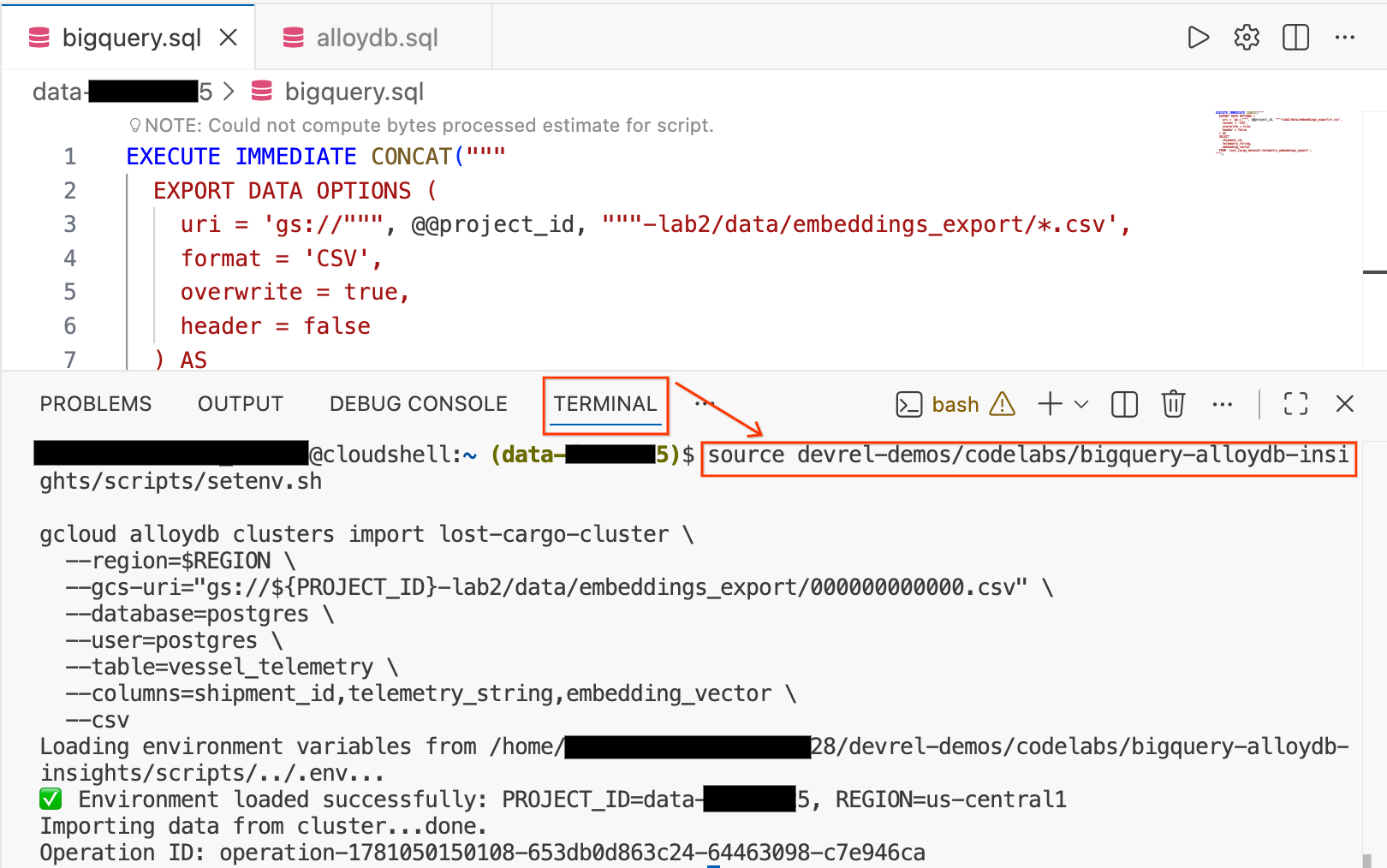
Use BigQuery's EXPORT DATA statement to write the embeddings table to your lab's GCS bucket as a CSV file.

EXECUTE IMMEDIATE CONCAT("""
  EXPORT DATA OPTIONS (
    uri = 'gs://""", @@project_id, """-lab2/data/embeddings_export/*.csv',
    format = 'CSV',
    overwrite = true,
    header = false
  ) AS
  SELECT
    shipment_id,
    telemetry_string,
    embedding_vector
  FROM `lost_cargo_dataset.telemetry_embeddings_export`;
""");

Step 4: Import into AlloyDB from Cloud Storage

1. In your Cloud Shell Editor, click the Terminal tab at the bottom of the screen to open a terminal session.
2. Run the following commands to load your environment and import the CSV file directly into the vessel_telemetry table in AlloyDB:

source devrel-demos/codelabs/bigquery-alloydb-insights/scripts/setenv.sh

gcloud alloydb clusters import lost-cargo-cluster \
  --region=$REGION \
  --gcs-uri="gs://${PROJECT_ID}-lab2/data/embeddings_export/000000000000.csv" \
  --database=postgres \
  --user=postgres \
  --table=vessel_telemetry \
  --columns=shipment_id,telemetry_string,embedding_vector \
  --csv

Section Recap: You used BigQuery's AI functions to summarize and embed the telemetry data, exported the results to Cloud Storage as CSV, then imported them into AlloyDB using gcloud. The operational tracking database is now loaded and ready.

8. Matching the Beacon Signal

A field team near Sydney has intercepted a fragmented telemetry beacon signal. The partial log reads:

"Refrigeration unit offline. Manual override."

If this came from the stolen container, AlloyDB's vector search should be able to match it even though the signal is incomplete. This is exactly the kind of real-time, operational query that AlloyDB is built for.

Step 1: Verify the Imported Data

Switch your editor tab back to alloydb.sql (which remains connected to AlloyDB).

Confirm that the telemetry data loaded successfully by running:

SELECT shipment_id, LEFT(telemetry_string, 80) AS telemetry_preview
FROM vessel_telemetry
LIMIT 10;

You should see rows with shipment_id values and telemetry text. These are the fleet's telemetry signatures, now ready for real-time matching.

Step 2: Search for the Missing Container

Now, use AlloyDB's google_ml_integration extension to search for a match using the intercepted signal fragment:

SELECT
    shipment_id,
    telemetry_string,
    1 - (embedding_vector <=> embedding('text-embedding-005', 'Refrigeration unit offline. Manual override.')::vector) AS search_relevance_score
FROM vessel_telemetry
ORDER BY embedding_vector <=> embedding('text-embedding-005', 'Refrigeration unit offline. Manual override.')::vector
LIMIT 5;

The embedding() function, provided by AlloyDB's google_ml_integration extension, calls Agent Platform directly from SQL to generate a vector embedding inline. The <=> operator calculates cosine distance between two vectors (the closer to 0, the more identical two vectors are). We subtract from 1 to express results as a relevance score where higher is better.

Same model, both databases. Notice that AlloyDB's embedding() function uses the same text-embedding-005 model that BigQuery's AI.EMBED used to generate the stored vectors. Because both call the same underlying Agent Platform embedding model, the embeddings are directly comparable, meaning a search vector generated in AlloyDB is mathematically compatible with vectors generated in BigQuery.

Step 3: Confirm the Match

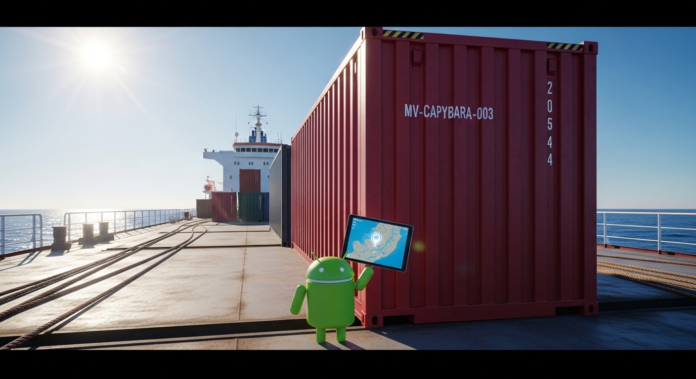
Examine the results. The top result should be MV-CAPYBARA-003, with the highest relevance score.

That's the same container you've been tracking across every step of this investigation:

• 📷 Security footage identified it leaving the Port of Rio de Janeiro at night.
• 🌡️ Thermal anomaly detection confirmed its refrigeration unit was deliberately disabled.
• 📡 Beacon signal matching just pinpointed its telemetry signature near Sydney.

Three independent lines of evidence. Three different Google Cloud AI capabilities. One stolen container.

🎯 Case closed: MV-CAPYBARA-003 has been located near Sydney!

🔍 Location Clue Unlocked: The AlloyDB vector search resolved the fragmented beacon signal with high confidence. You have unlocked the container's location: it has been located at the docks near Sydney!

Section Recap: You used AlloyDB's built-in AI integration to generate a search embedding and perform a cosine similarity search in a single SQL query. The beacon match confirmed the stolen container's location, completing the investigation.

9. Exploring the Evidence

Now that you've identified the container through multimodal image analysis and vector search, you can use Conversational Analytics directly inside your editor to explore the investigation data using natural language, without writing any SQL.

Step 1: Locate the Data in Knowledge Catalog

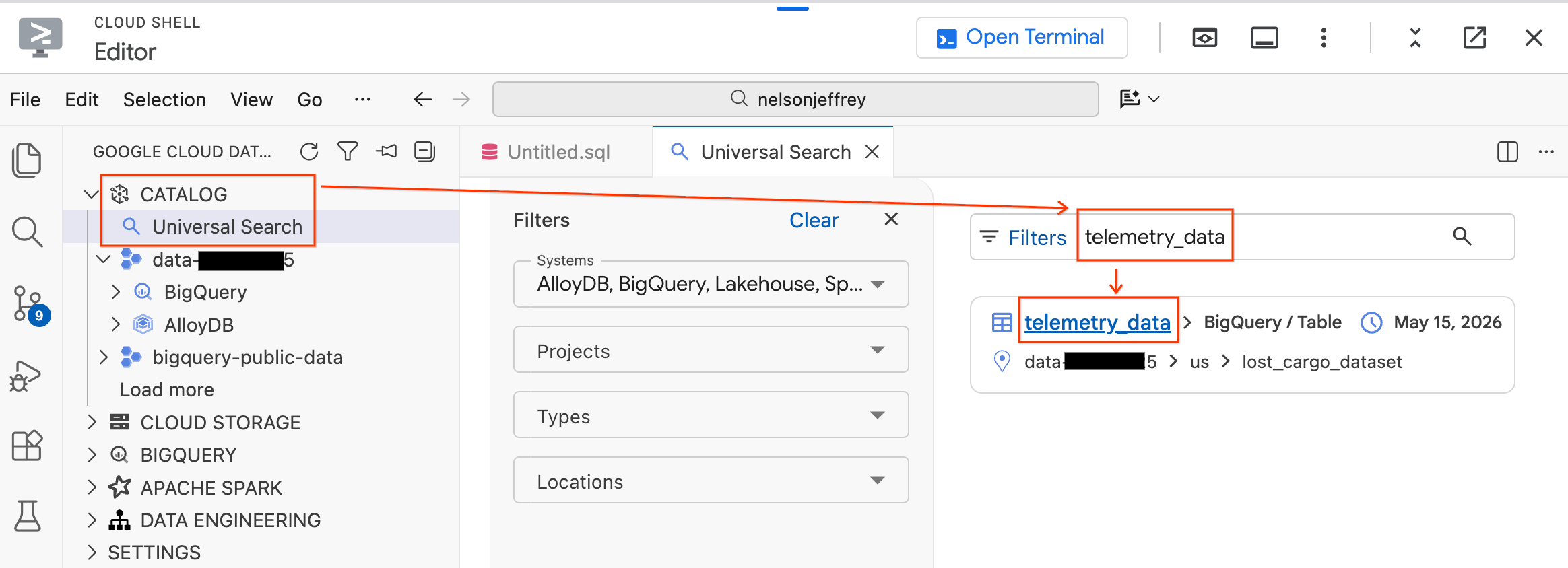
The Data Agent Kit includes a Universal Search feature that lets you find and explore data assets across your Google Cloud environment.

1. In the Data Agent Kit panel on the left, expand the Catalog section.
2. Click Universal Search.
3. In the search bar, type telemetry_data.
4. Click on the telemetry_data table (under lost_cargo_dataset) from the search results.

Step 2: Launch Conversational Analytics

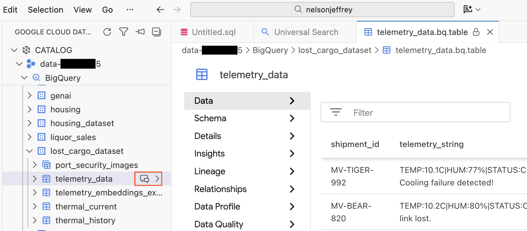
Clicking the search result opens a data viewer tab where you can preview the raw data, view the schema, and check data quality.

1. On the left pane, your BigQuery datasets and tables are visible. Click the Chat button to open up a new chat window.

Step 3: Ask Questions in Natural Language

A new "Welcome to Conversational Analytics!" chat tab opens. The agent has context about your table's schema and contents.

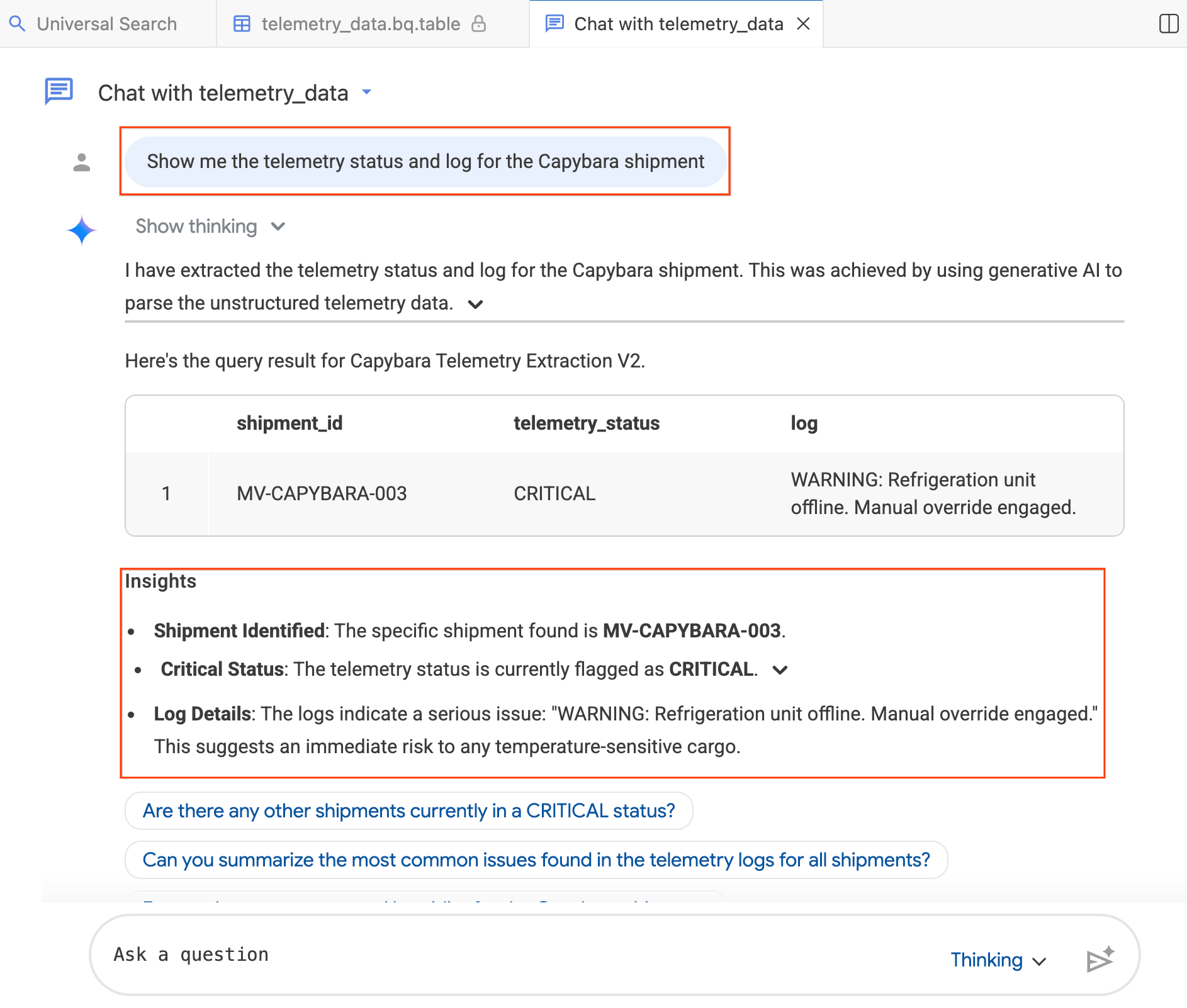
1. In the chat window, type:"Show me the telemetry status and log for the Capybara shipment."
2. Press Enter.

The agent translates your question into BigQuery SQL, executes the query, and returns the results, including both a data table and Insights summarizing the findings. You can toggle between Thinking (deeper analysis, slower) and Fast (quicker responses) mode depending on the complexity of your question. Since these are AI-generated responses, your results may look slightly different from the screenshots below.

Step 4: Ask Follow-up Questions

The agent remembers the context of your conversation. Try a follow-up question:

• "How many unique shipments are in the telemetry data?"
• "How many other shipments in the fleet currently have a CRITICAL status?"

What is Conversational Analytics? Conversational Analytics translates natural language into executable SQL and summarizes the results, making data analysis accessible to investigators and analysts, not just SQL experts.

Section Recap: You used Knowledge Catalog's Universal Search feature to locate your dataset and launched Conversational Analytics to query investigation data with natural language. The AI agent translated your questions into SQL and provided insights that corroborated your findings.

10. Clean Up

To avoid incurring ongoing charges to your Google Cloud account, delete the resources you created in this lab. You can run these commands in your integrated terminal inside the Cloud Shell Editor (where you've been using the Data Agent Kit) to clean up your environment.

First, load your environment variables:

source scripts/setenv.sh

1. Delete BigQuery Resources (only if you are not continuing to Lab 3):

If you plan to continue to Lab 3, skip this step! Lab 3 uses the same BigQuery dataset and connections for property graph analytics.

To delete your BigQuery dataset and connections:

# Drop the dataset
bq rm -r -f $PROJECT_ID:lost_cargo_dataset

# Delete the connections
bq rm --connection --location=us-central1 $PROJECT_ID.us-central1.lost_cargo_conn
bq rm --connection --location=us-central1 $PROJECT_ID.us-central1.lost_cargo_alloydb_conn

2. Delete the Cloud Storage bucket:

gcloud storage rm --recursive gs://${PROJECT_ID}-lab2

3. Delete the AlloyDB instance and cluster:

AlloyDB is not used in Lab 3, so it is safe to tear it down now.

gcloud alloydb instances delete lost-cargo-instance \
  --region=$REGION \
  --cluster=lost-cargo-cluster \
  --quiet

gcloud alloydb clusters delete lost-cargo-cluster \
  --region=$REGION \
  --force \
  --quiet

4. Delete the local environment settings:

Finally, clean up the local environment settings file from your workspace:

rm -f .env

11. Congratulations!

You've successfully completed Lab 2: Data Analysis & Multimodal Insights! You followed the trail from a port full of thousands of containers to a confirmed theft and a pinpointed location.

What you accomplished

1. Scanned the footage: You used BigQuery's AI.GENERATE to analyze port security images and identify container MV-CAPYBARA-003 in Crimson Red.
2. Confirmed the theft: You explored thermal sensor data, spotted a suspicious 148.4°F spike, and used AI.DETECT_ANOMALIES to prove it was deliberate tampering.
3. Prepared the tracking system: You configured AlloyDB with pgvector and google_ml_integration for real-time beacon matching.
4. Built the search index: You used AI.GENERATE and AI.EMBED in BigQuery to create embeddings, then exported them to Cloud Storage and imported them into AlloyDB.
5. Matched the beacon signal: You used AlloyDB's vector search to match a fragmented telemetry signal, locating the stolen container near Sydney.
6. Explored the evidence: You used Conversational Analytics directly from the editor to query investigation data with natural language.

Next Steps

You've found where the container is. Now you need to find out who is behind it.

In Lab 3: Data Consumption & Agentic Workflows, you'll build a property graph of the logistics network to map relationships between shell companies, use Conversational Analytics to chat with the graph, and hunt through Knowledge Catalog to find the secured clearance code needed to recover the container.