Lab 3: Uncovering Lost Cargo with BigQuery Graph and Conversational Analytics

1. Introduction

Welcome to the final stage of the Lost Cargo investigation! After tracking the stolen container of Android figurines from London all the way to Sydney, the trail has gone cold. By disabling its transponder, the container's smart security vault has triggered an automatic emergency lockdown.

To recover the high-value cargo before it is locked forever, your mission is to find the container's final location and retrieve the manual override passcode to physically unlock the vault.

To find the missing container and secure the cargo, you will build a BigQuery Property Graph to trace the shipment's journey. You will then query this network in natural language using Conversational Analytics, and finish up by performing a semantic search over your data's metadata with Knowledge Catalog to locate the override codes.

💡 Missed Lab 1 or Lab 2? Don't worry! This lab is fully self-contained. The environment setup steps will provision everything you need so you can jump straight in and complete it independently.

What you'll do

• Clone the repository and run the setup script in Google Cloud Shell.
• Build a Property Graph in BigQuery linking company, vessel, and manifest data.
• Use Conversational Analytics to query the graph in natural language, tracing the cargo's journey to identify the responsible operator.
• Locate the table holding the final override codes using Knowledge Catalog.
• Use BigQuery Column level access control to unmask and reveal the final code.

What you'll need

• A web browser such as Chrome
• A Google Cloud project with billing enabled
• Access to Google Cloud Shell

This codelab is designed for data practitioners of all levels.

The resources created in this codelab should cost less than $5.

Estimated duration: This codelab will take approximately 45 minutes to complete.

2. Before you begin

Create a Google Cloud Project

1. In the Google Cloud Console, on the project selector page, select or create a Google Cloud project.
2. Make sure that billing is enabled for your Cloud project.

Start Cloud Shell

You will use Google Cloud Shell to download the code, run setup scripts, and deploy the application.

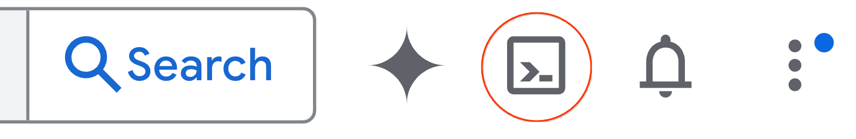
1. In a new browser tab, open the Cloud Shell:

2. Once connected, set your project ID and confirm your environment:

gcloud config set project <<YOUR_PROJECT_ID>>
export PROJECT_ID=$(gcloud config get-value project)
export REGION=us-central1

You should see a message similar to:

Your active configuration is: [cloudshell-####]
Updated property [core/project]

Enable Required APIs

Run the following command in Cloud Shell to enable the required APIs:

gcloud services enable \
 bigquery.googleapis.com \
 aiplatform.googleapis.com \
 datacatalog.googleapis.com  \
 geminidataanalytics.googleapis.com \
 cloudaicompanion.googleapis.com 

On successful execution, you should see a message similar to:

Operation "operations/..." finished successfully.

3. Set Up Your Environment

In the previous labs of this series, we laid the groundwork for our investigation.

1. Clone the repository

Clone the codelab repository to your Cloud Shell environment:

cd ~/
git clone --filter=blob:none --no-checkout https://github.com/GoogleCloudPlatform/devrel-demos.git
cd ~/devrel-demos
git sparse-checkout init --cone
git sparse-checkout set codelabs/bigquery-graph-analytics
git checkout main
cd codelabs/bigquery-graph-analytics/

2. Set up base tables and policy tags

Run the setup script to populate your BigQuery dataset and apply column-level security tags to restrict sensitive data:

bash setup_lab.sh

Confirm that the output in your terminal shows successful initialization:

🚀 Provisioning foundational tables and deploying Policy Tag security bindings...
🎯 Active Project: your-project-id
...
🎉 Success! Foundational tables initialized and Column-Level Policy Tags fully mapped out of the box!

With your environment successfully set up and the logistics data populated BigQuery, you can now build a Property Graph to connect your tables and trace the cargo's journey!

4. Connect your data using BigQuery Graph

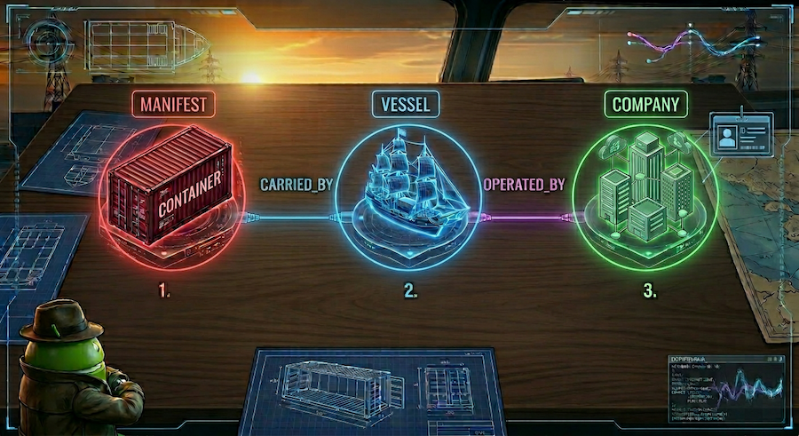
To analyze our supply chain data, we will define how companies, vessels, and manifests relate to one another. Building a property graph allows us to query these connections easily.

1. How Property Graphs Model Relationships

A BigQuery property graph models networks using:

• Nodes: The entities in the network. In this lab, nodes represent Companies (which store contact details directly), Manifests, and Vessels.
• Edges: The relationships linking nodes together. For example:
  • An edge connects a Manifest to a Vessel (via relationships in the manifests table).
  • An edge connects a Vessel to a Company (via relationships in the vessels table).
• Properties: Metadata stored on nodes or edges. For example, a Company node has columns like company_name and phone_number, and a Manifest node has seal_integrity_status and coordinates (last_ping_lat, last_ping_long).
• Labels: Tag names assigned to nodes (e.g., Company, Vessel, Manifest) and edges (e.g., CARRIED_BY, OPERATED_BY) so query tools can recognize node and relation types.

2. Deploy the Property Graph in BigQuery

The setup_graph.sql file contains the SQL DDL to define and create the property graph, but it is currently incomplete. You need to define the edge labels (relationships) in this schema file before compiling and deploying it:

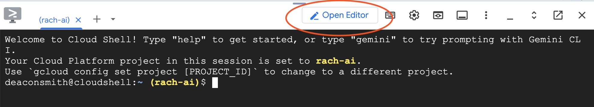
1. Open the Cloud Shell Editor.

2. Open the file setup_graph.sql in the Cloud Shell Editor.

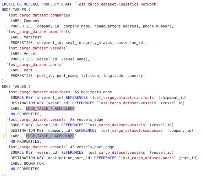
3. Locate the placeholders for edge labels:
   • Line 22: Replace `EDGE_TABLE_PLACEHOLDER` with a meaningful tag representing how manifests relate to vessels (e.g., CARRIED_BY).
   • Line 27: Replace `EDGE_TABLE_PLACEHOLDER` with a tag representing how vessels relate to companies (e.g., OPERATED_BY).
4. Save the file.

Now, return to Cloud Shell terminal and deploy the updated property graph using the completed script:

bq query --use_legacy_sql=false < setup_graph.sql

You should see output indicating that the job is complete:

Waiting on bqjob_r... ... (0s) Current status: DONE

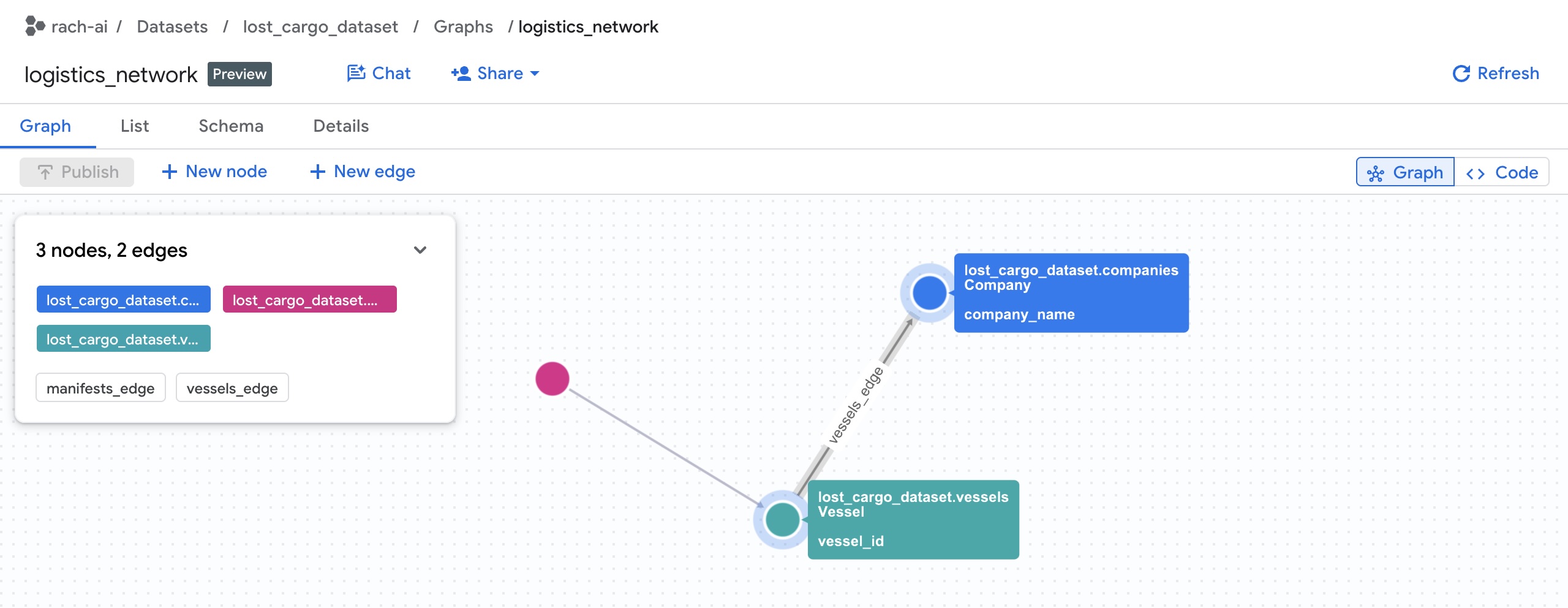
You can view the Property Graph details in the BigQuery Console:

Find the lost_cargo_dataset and select Graphs:

With our property graph successfully compiled, let's dive into BigQuery Studio to query and visualize the connections!

5. Query your Graph

You can query and explore the graph visually using native Graph Query Language (GQL) directly inside BigQuery Studio.

1. Query the container -> vessel -> company chain

Let's explore GQL queries by finding who operates the vessels carrying cargo. Finding the operator requires traversing across three separate entity nodes in our logistics network:

1. Start at the container Manifest node.
2. Follow the CARRIED_BY relationship edge to find the carrying Vessel.
3. Follow the OPERATED_BY relationship edge from that vessel to the responsible Company and retrieve its ID.

First, let's run a query to visualize the entire network (without any filters) to see the full graph.

1. Open a new tab in the BigQuery Studio SQL editor, paste the following GQL query, and click Run:

   SELECT * FROM GRAPH_TABLE(
     `lost_cargo_dataset.logistics_network`
     MATCH p = (m:Manifest)-[:CARRIED_BY]->(v:Vessel)-[:OPERATED_BY]->(comp:Company)
     RETURN TO_JSON(p) AS path
   );
   

2. When the query completes, in the Query results pane at the bottom, click the Graph tab (located next to the Results table tab).

3. BigQuery renders the results as an interactive visual graph representation! Zoom in to see the full network of connected containers, vessels, and operators.

Anatomy of a GQL Query

Let's breakdown the GQL query we just ran:

• GRAPH_TABLE: Directs BigQuery to execute a property graph query against the logistics_network graph.
• MATCH: Declares the multi-hop traversal pattern. We start at a Manifest (m), match the edge relationship :CARRIED_BY pointing to Vessel (v), then match the edge relationship :OPERATED_BY pointing to Company (comp).
• GQL replaces complex join logic with intuitive, human-readable ASCII-art relationship arrows ()->[]->(), making it super simple to write and optimize multi-hop queries.
• RETURN: Returns properties or the JSON path from the matched elements.

2. Filter GQL query results

Now, let's filter the query so that we only look at the path for our target compromised container MV-CAPYBARA-003.

1. Paste the following query into the SQL editor and click Run:

   SELECT * FROM GRAPH_TABLE(
     `lost_cargo_dataset.logistics_network`
     MATCH p = (m:Manifest {shipment_id: 'MV-CAPYBARA-003'})-[:CARRIED_BY]->(v:Vessel)-[:OPERATED_BY]->(comp:Company)
     RETURN TO_JSON(p) AS path
   );
   

2. Click the Graph tab under results.

3. The viewer now displays only the active traversal route for MV-CAPYBARA-003. Zoom in to see the nodes and connections:
   • Double-click the Company node to open the properties panel. Under Properties, you will see the operator company_id: 103 (Davy Jones Shipping). Note down this company ID—you will need it later to retrieve the clearance passcode from the security registry!
   • Double-click the Vessel node to verify it is the Flying Dutchman.

Status Check:

• What we achieved: Queried our property graph network to locate the operator of the vessel carrying the missing shipment (company_id: 103 / Davy Jones Shipping).
• What we need to do next: Explore our graph further to locate where the compromised vessel is heading.

6. Chat with your Graph using Conversational Analytics

Now that you've queried your graph manually to find the company ID, let's use Conversational Analytics to chat directly with our graph and pinpoint where our container is headed.

1. Start a Conversational Analytics session

1. In the Google Cloud Console, navigate to the BigQuery Console, and expand the resources panel to find your dataset (lost_cargo_dataset).
2. Click on your Property Graph resource: logistics_network.
3. In the detail panel toolbar at the top, click the Chat button. This opens a Conversational Analytics session pre-loaded with the context of your graph.

Tip: The Conversational Analytics agent automatically reads your graph structure, pre-loading its context when you click Chat.

2. Pinpoint the nearest docking port for the hijacked container

A marine patrol aircraft has just spotted a vessel matching our cargo ship's description sailing off-grid (with its transponder deactivated) at coordinates POINT(-122.48 37.55). To intercept the cargo, we need to find the nearest docking port where the shadow syndicate Davy Jones Shipping operates.

Instead of manually searching all global ports, we will query our graph network to pull the ports connected to the syndicate's active fleet and measure which one is physically closest to the sighting!

1. In the Conversational Analytics chat box, enter the following prompt:

   Find all ports associated with Davy Jones Shipping vessels. Which port is closest to coordinate POINT(-122.48 37.55), show the distance in km, and display it on a map.
   

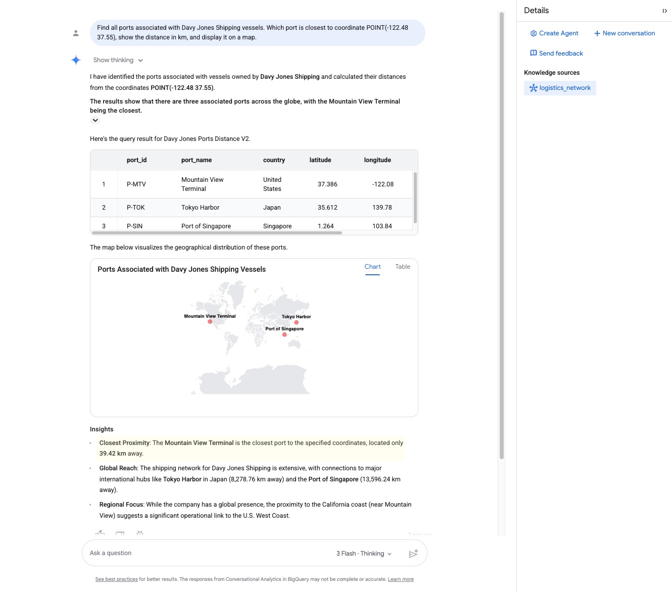
2. Look closely at the response. The agent traverses the graph and returns the closest docking facility and its distance:
   • Docking Port: Mountain View Terminal
   • Distance: 39.42 kilometers
3. Because Conversational Analytics is powered by Gemini with native geospatial (GIS) integration, it can interpret geography coordinate points and leverage its world knowledge to verify the location:"The vessel is approximately 39.42 kilometers from Mountain View Terminal, California, indicating it is heading there to dock."

This confirms our cargo is heading directly to Mountain View!

Under the hood: Graph Query Language (GQL) & Geospatial GIS

Behind the scenes, the Conversational Analytics agent dynamically compiled and executed a query that combines Graph path matching with Geospatial distance calculations. This is achieved using a native GQL COLUMNS clause, computing the geodesic distance natively inside the graph traversal match:

SELECT port_id, port_name, country, latitude, longitude, distance_km 
FROM GRAPH_TABLE(
  `lost_cargo_dataset.logistics_network`
  MATCH (c:Company)<-[]-(v:Vessel)-[]->(p:Port)
  WHERE LOWER(c.company_name) = 'davy jones shipping'
  COLUMNS (
    p.port_id, 
    p.port_name, 
    p.country, 
    p.latitude, 
    p.longitude, 
    ROUND(ST_DISTANCE(ST_GEOGPOINT(p.longitude, p.latitude), ST_GEOGPOINT(-122.48, 37.55)) / 1000, 2) AS distance_km
  )
)
ORDER BY distance_km ASC;

By combining native Geospatial (GIS) functions (ST_DISTANCE, ST_GEOGPOINT) with a GQL property graph match, BigQuery dynamically resolves the syndicate's operational footprint and computes real-world physical proximity in a single query!

Status Check:

• What we achieved: Used Conversational Analytics to trace the shadow operator's fleet docking ports (Manifest ➔ Vessel ➔ Company ➔ Docks) and calculated that the suspect ship is heading directly to the Mountain View Terminal (only ~39 km away).
• What we need to do next: Find the data registry that contains the manual override code so our local tactical intervention squad can intercept the shipment and manually unlock the container once it docks at the Mountain View Terminal!

7. Find your missing data with Knowledge Catalog

The property graph shows relationships, but it does not contain the table where the actual override codes are stored.

In a real enterprise environment with hundreds of datasets and tables, finding this information can be difficult. We will use Knowledge Catalog to perform a semantic search and locate the correct table.

1. Semantic Search in Knowledge Catalog

1. In the Google Cloud Console, search for and navigate to Knowledge Catalog ➔ Search.
2. In the search filter column under Systems, check BigQuery to narrow down results.
3. In the search box, enter the following query:

   container override codes
   

4. Click on the maritime_security_registry table resource that appears in the search results:

Upon inspecting the metadata schema, you will see the table holds columns for container security data—such as the coordinator company co_id, custodian token cust_tok, and most importantly, the secure container override passcode column: clc_ovr_cd.

We have successfully located both the table and the exact secure column we need to recover our cargo!

Under the Hood: Semantic Matching: The table name (maritime_security_registry) and its key column name (clc_ovr_cd) are completely obscure. Without Knowledge Catalog's semantic search parsing the column description ("Secure container override passcode"), finding this table by searching for "override codes" would have been nearly impossible.

🔓 Real-World Governance: In a production enterprise environment, security and governance teams also leverage:

• Aspects and Tag Templates: To attach business metadata (such as Data Owner, Retention Period, or PII Classification) to table schemas.
• Data Lineage: To auto-generate visual flowcharts representing how tables like maritime_security_registry are queried and consumed by downstream systems.

2. Inspect Column Security in BigQuery

1. Navigate back to the BigQuery Console.
2. In the Explorer tab, select the lost_cargo_dataset and click the maritime_security_registry table.
3. Click on the Schema tab.

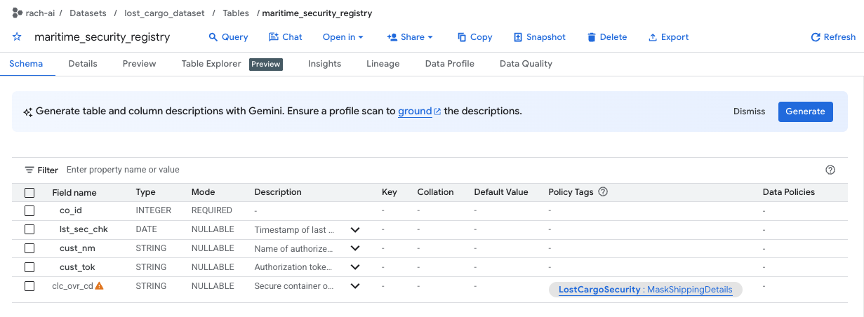
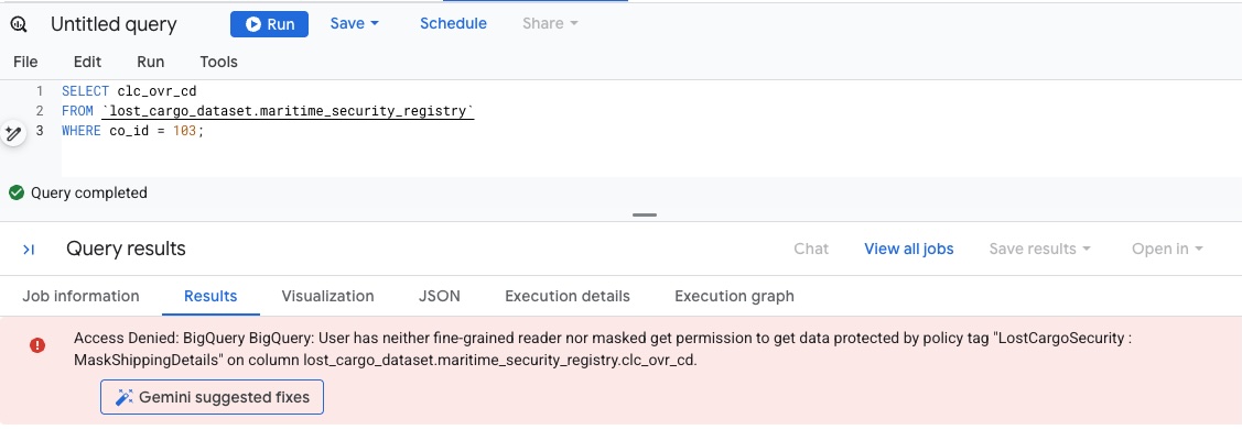
4. Notice that the clc_ovr_cd column is secured by a policy tag named MaskShippingDetails (listed in the Policy tags column).
5. Open a new SQL Editor tab in BigQuery and attempt to view the registry override codes by running the following query:

   SELECT * FROM `lost_cargo_dataset.maritime_security_registry` 
   WHERE co_id = 103;
   

6. Because your account does not yet have permissions to read columns tagged with MaskShippingDetails, the query will fail immediately with an Access Denied database security error:

Status Check:

• What we achieved: Found the secure table (maritime_security_registry) and column (clc_ovr_cd) holding the override code.
• What we need to do next: Grant your account read permissions for the secured column.

8. Cracking Column Security to Retrieve the Passcode

To read the final override code in clear-text, we need to grant our user account permission to read columns tagged with MaskShippingDetails.

1. Grant Policy Tag Permissions

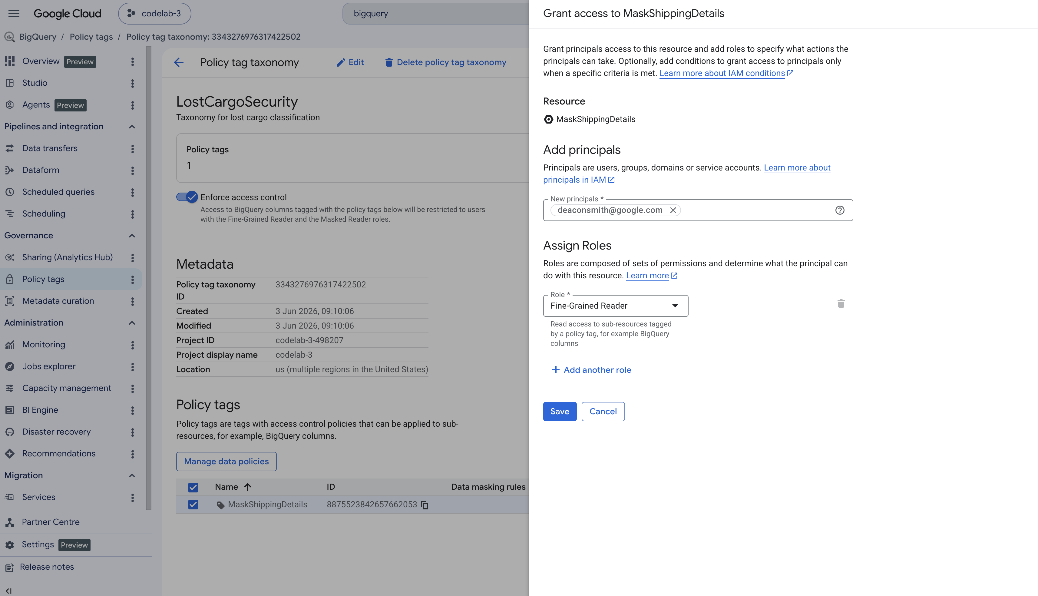
1. In the BigQuery console left navigation pane, navigate to Policy tags.
2. Select the taxonomy named LostCargoSecurity_.
3. In the list of tags, click MaskShippingDetails.
4. In the Info panel on the right side of the screen, click Add Principal. (If the panel is hidden, click Show Info Panel in the top right).
5. In the New principals field, enter your active Google Cloud user email.
6. In the Select a role dropdown, search for and select Fine-Grained Reader, then click Save.

2. Query for the Override Code

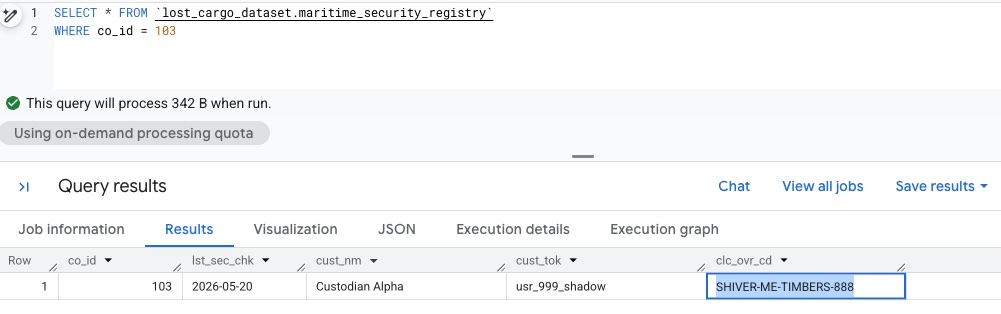
Go back to your BigQuery workspace editor. Because you now have fine-grained reader access, we should be able to run the query again and be able to see the unmasked data:

SELECT *  FROM `lost_cargo_dataset.maritime_security_registry` 
WHERE co_id = 103;

🔓 Result

The query returns the unmasked override code:

SHIVER-ME-TIMBERS-888

Mission Accomplished! 🚢

Congratulations! By combining BigQuery property graphs & Conversational Analytics with Knowledge Catalog and Column-Level Security, you successfully tracked the shadow fleet and extracted the secure container override code!.

The tactical interception team has been dispatched to the Mountain View Terminal! Armed with the decrypted override code, they are ready to unlock the Capybara container, secure the cargo, and successfully reclaim our lost assets.

9. Clean up

To avoid incurring charges, clean up the sandbox resources created during this lab.

Return to Cloud Shell Terminal and delete the BigQuery dataset containing the logistics tables:

bq rm -r -f -d lost_cargo_dataset

Remove the cloned repository files:

cd ..
rm -rf data-cloud-roadshow-26

10. Congratulations

You have successfully resolved the investigation and retrieved the clearance override code!

What you've learned

• How to build a property graph in BigQuery to represent complex entities and relationships.
• How Nodes, Edges, Properties, and Labels are configured to capture data connections.
• How to query property graphs using natural language with BigQuery Conversational Analytics.
• How Graph Query Language (GQL) expressions are structured to traverse relational paths.
• How to discover secured assets using Knowledge Catalog and access column-level restricted data using policy tags.

Resource Links

• BigQuery Conversational Analytics Overview
• BigQuery Property Graphs Syntax Reference
• Knowledge Catalog Integration