1. Overview
In this lab, you will learn how to assemble convolutional layer into a neural network model that can recognize flowers. This time, you will build the model yourself from scratch and use the power of TPU to train it in seconds and iterate on its design.
This lab includes the necessary theoretical explanations about convolutional neural networks and is a good starting point for developers learning about deep learning.
This lab is Part 3 of the "Keras on TPU" series. You can do them in the following order or independently.
- TPU-speed data pipelines: tf.data.Dataset and TFRecords
- Your first Keras model, with transfer learning
- [THIS LAB] Convolutional neural networks, with Keras and TPUs
- Modern convnets, squeezenet, Xception, with Keras and TPUs
What you'll learn
- To build a convolutional image classifier using a Keras Sequential model.
- To train your Keras model on TPU
- To fine-tune your model with a good choice of convolutional layers.
Feedback
If you see something amiss in this code lab, please tell us. Feedback can be provided through GitHub issues [ feedback link].
2. Google Colaboratory quick start
This lab uses Google Collaboratory and requires no setup on your part. Colaboratory is an online notebook platform for education purposes. It offers free CPU, GPU and TPU training.

You can open this sample notebook and run through a couple of cells to familiarize yourself with Colaboratory.
Select a TPU backend
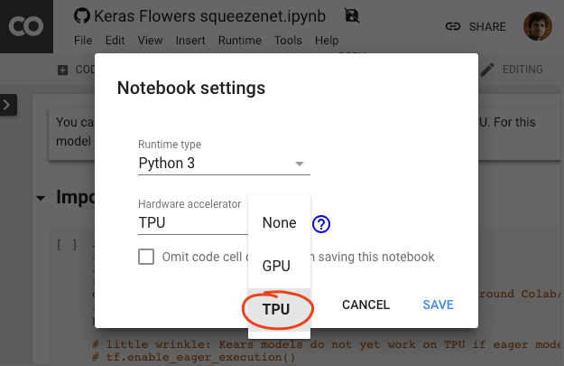
In the Colab menu, select Runtime > Change runtime type and then select TPU. In this code lab you will use a powerful TPU (Tensor Processing Unit) backed for hardware-accelerated training. Connection to the runtime will happen automatically on first execution, or you can use the "Connect" button in the upper-right corner.
Notebook execution

Execute cells one at a time by clicking on a cell and using Shift-ENTER. You can also run the entire notebook with Runtime > Run all
Table of contents

All notebooks have a table of contents. You can open it using the black arrow on the left.
Hidden cells

Some cells will only show their title. This is a Colab-specific notebook feature. You can double click on them to see the code inside but it is usually not very interesting. Typically support or visualization functions. You still need to run these cells for the functions inside to be defined.
Authentication

It is possible for Colab to access your private Google Cloud Storage buckets provided you authenticate with an authorized account. The code snippet above will trigger an authentication process.
3. [INFO] What are Tensor Processing Units (TPUs) ?
In a nutshell

The code for training a model on TPU in Keras (and fall back on GPU or CPU if a TPU is not available):
try: # detect TPUs
    tpu = tf.distribute.cluster_resolver.TPUClusterResolver.connect()
    strategy = tf.distribute.TPUStrategy(tpu)
except ValueError: # detect GPUs
    strategy = tf.distribute.MirroredStrategy() # for CPU/GPU or multi-GPU machines

# use TPUStrategy scope to define model
with strategy.scope():
  model = tf.keras.Sequential( ... )
  model.compile( ... )

# train model normally on a tf.data.Dataset
model.fit(training_dataset, epochs=EPOCHS, steps_per_epoch=...)
We will use TPUs today to build and optimize a flower classifier at interactive speeds (minutes per training run).

Why TPUs ?
Modern GPUs are organized around programmable "cores", a very flexible architecture that allows them to handle a variety of tasks such as 3D rendering, deep learning, physical simulations, etc.. TPUs on the other hand pair a classic vector processor with a dedicated matrix multiply unit and excel at any task where large matrix multiplications dominate, such as neural networks.
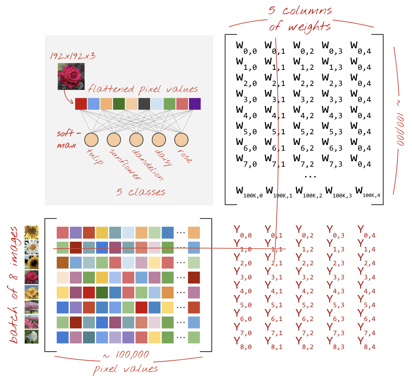
Illustration: a dense neural network layer as a matrix multiplication, with a batch of eight images processed through the neural network at once. Please run through one line x column multiplication to verify that it is indeed doing a weighted sum of all the pixels values of an image. Convolutional layers can be represented as matrix multiplications too although it's a bit more complicated ( explanation here, in section 1).
The hardware
MXU and VPU
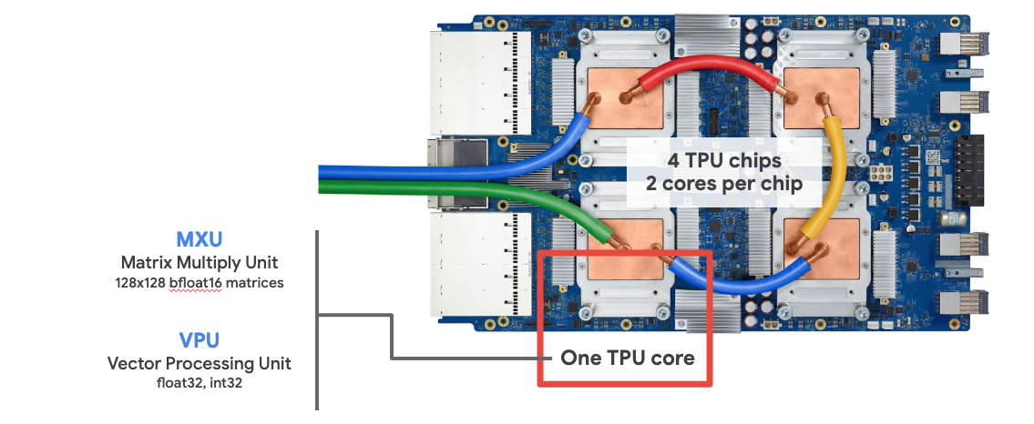
A TPU v2 core is made of a Matrix Multiply Unit (MXU) which runs matrix multiplications and a Vector Processing Unit (VPU) for all other tasks such as activations, softmax, etc. The VPU handles float32 and int32 computations. The MXU on the other hand operates in a mixed precision 16-32 bit floating point format.
Mixed precision floating point and bfloat16
The MXU computes matrix multiplications using bfloat16 inputs and float32 outputs. Intermediate accumulations are performed in float32 precision.
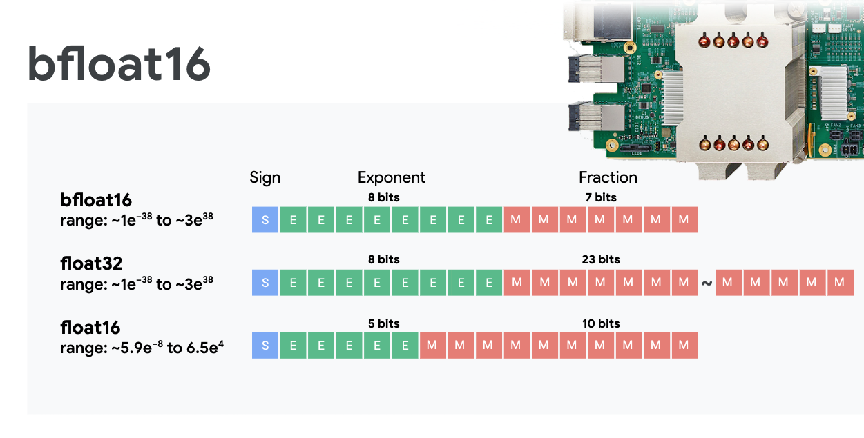
Neural network training is typically resistant to the noise introduced by a reduced floating point precision. There are cases where noise even helps the optimizer converge. 16-bit floating point precision has traditionally been used to accelerate computations but float16 and float32 formats have very different ranges. Reducing the precision from float32 to float16 usually results in over and underflows. Solutions exist but additional work is typically required to make float16 work.
That is why Google introduced the bfloat16 format in TPUs. bfloat16 is a truncated float32 with exactly the same exponent bits and range as float32. This, added to the fact that TPUs compute matrix multiplications in mixed precision with bfloat16 inputs but float32 outputs, means that, typically, no code changes are necessary to benefit from the performance gains of reduced precision.
Systolic array
The MXU implements matrix multiplications in hardware using a so-called "systolic array" architecture in which data elements flow through an array of hardware computation units. (In medicine, "systolic" refers to heart contractions and blood flow, here to the flow of data.)
The basic element of a matrix multiplication is a dot product between a line from one matrix and a column from the other matrix (see illustration at the top of this section). For a matrix multiplication Y=X*W, one element of the result would be:
Y[2,0] = X[2,0]*W[0,0] + X[2,1]*W[1,0] + X[2,2]*W[2,0] + ... + X[2,n]*W[n,0]
On a GPU, one would program this dot product into a GPU "core" and then execute it on as many "cores" as are available in parallel to try and compute every value of the resulting matrix at once. If the resulting matrix is 128x128 large, that would require 128x128=16K "cores" to be available which is typically not possible. The largest GPUs have around 4000 cores. A TPU on the other hand uses the bare minimum of hardware for the compute units in the MXU: just bfloat16 x bfloat16 => float32 multiply-accumulators, nothing else. These are so small that a TPU can implement 16K of them in a 128x128 MXU and process this matrix multiplication in one go.
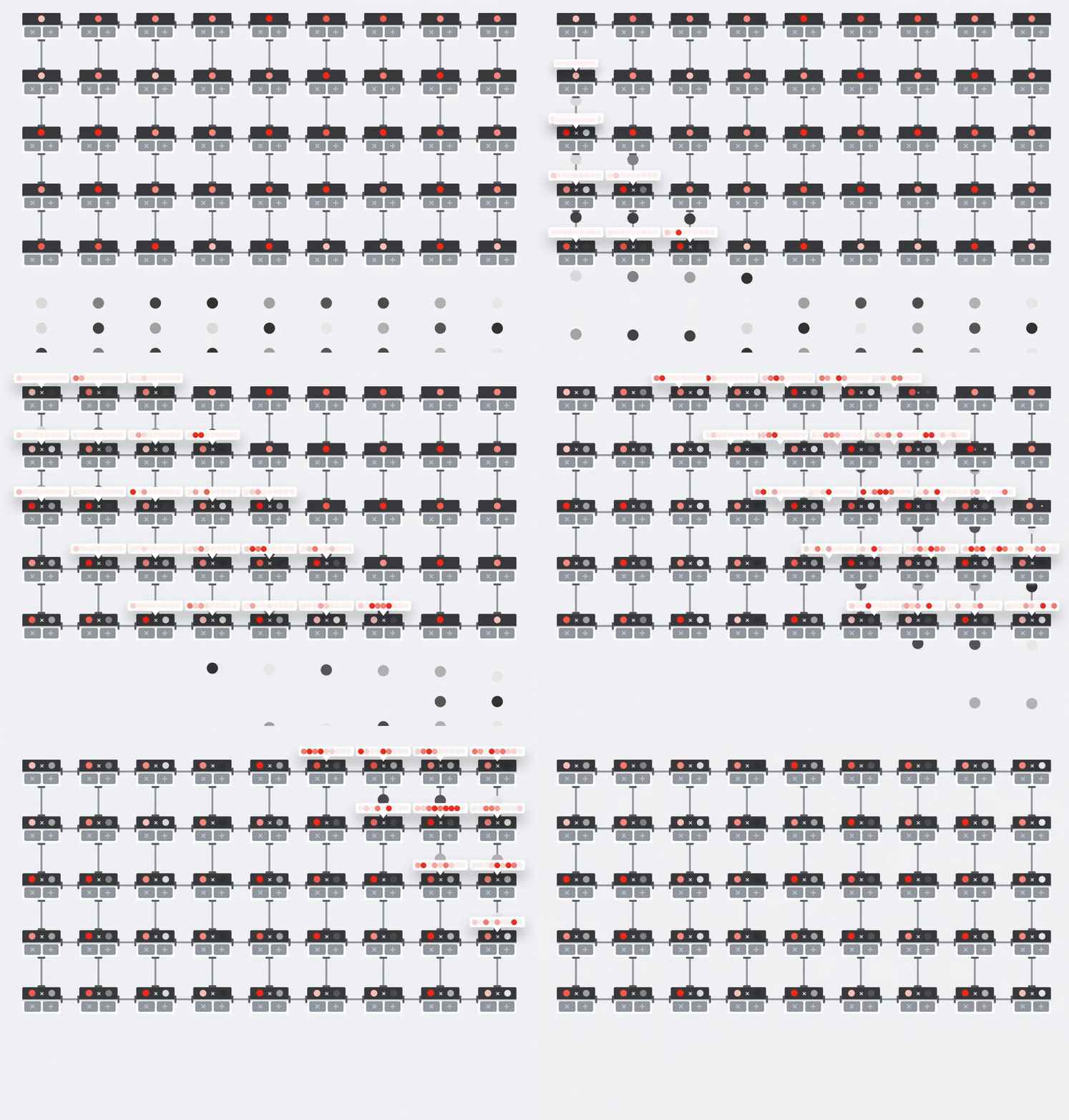
Illustration: the MXU systolic array. The compute elements are multiply-accumulators. The values of one matrix are loaded into the array (red dots). Values of the other matrix flow through the array (grey dots). Vertical lines propagate the values up. Horizontal lines propagate partial sums. It is left as an exercise to the user to verify that as the data flows through the array, you get the result of the matrix multiplication coming out of the right side.
In addition to that, while the dot products are being computed in an MXU, intermediate sums simply flow between adjacent compute units. They do not need to be stored and retrieved to/from memory or even a register file. The end result is that the TPU systolic array architecture has a significant density and power advantage, as well as a non-negligible speed advantage over a GPU, when computing matrix multiplications.
Cloud TPU
When you request one " Cloud TPU v2" on Google Cloud Platform, you get a virtual machine (VM) which has a PCI-attached TPU board. The TPU board has four dual-core TPU chips. Each TPU core features a VPU (Vector Processing Unit) and a 128x128 MXU (MatriX multiply Unit). This "Cloud TPU" is then usually connected through the network to the VM that requested it. So the full picture looks like this:
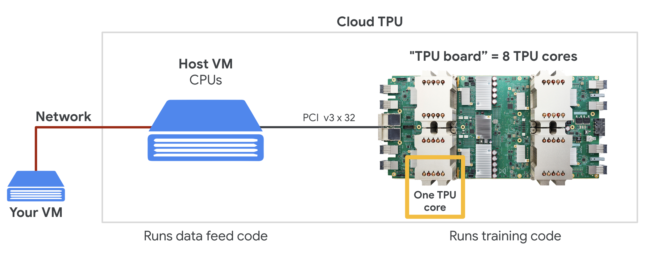
Illustration: your VM with a network-attached "Cloud TPU" accelerator. "The Cloud TPU" itself is made of a VM with a PCI-attached TPU board with four dual-core TPU chips on it.
TPU pods
In Google's data centers, TPUs are connected to a high-performance computing (HPC) interconnect which can make them appear as one very large accelerator. Google calls them pods and they can encompass up to 512 TPU v2 cores or 2048 TPU v3 cores..

Illustration: a TPU v3 pod. TPU boards and racks connected through HPC interconnect.
During training, gradients are exchanged between TPU cores using the all-reduce algorithm ( good explanation of all-reduce here). The model being trained can take advantage of the hardware by training on large batch sizes.
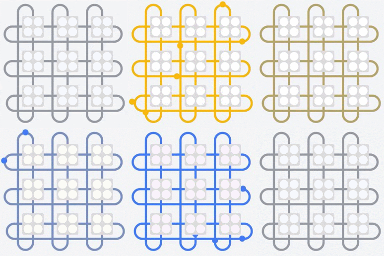
Illustration: synchronization of gradients during training using the all-reduce algorithm on Google TPU's 2-D toroidal mesh HPC network.
The software
Large batch size training
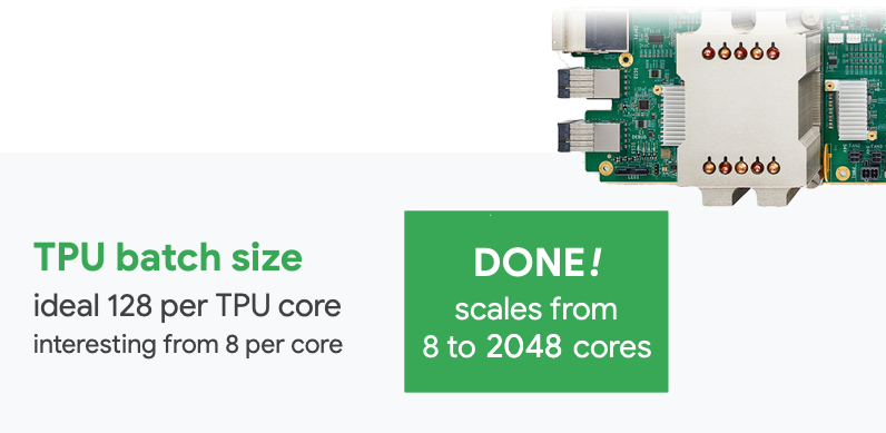
The ideal batch size for TPUs is 128 data items per TPU core but the hardware can already show good utilization from 8 data items per TPU core. Remember that one Cloud TPU has 8 cores.
In this code lab, we will be using the Keras API. In Keras, the batch you specify is the global batch size for the entire TPU. Your batches will automatically be split in 8 and ran on the 8 cores of the TPU.
For additional performance tips see the TPU Performance Guide. For very large batch sizes, special care might be needed in some models, see LARSOptimizer for more details.
Under the hood: XLA
Tensorflow programs define computation graphs. The TPU does not directly run Python code, it runs the computation graph defined by your Tensorflow program. Under the hood, a compiler called XLA (accelerated Linear Algebra compiler) transforms the Tensorflow graph of computation nodes into TPU machine code. This compiler also performs many advanced optimizations on your code and your memory layout. The compilation happens automatically as work is sent to the TPU. You do not have to include XLA in your build chain explicitly.
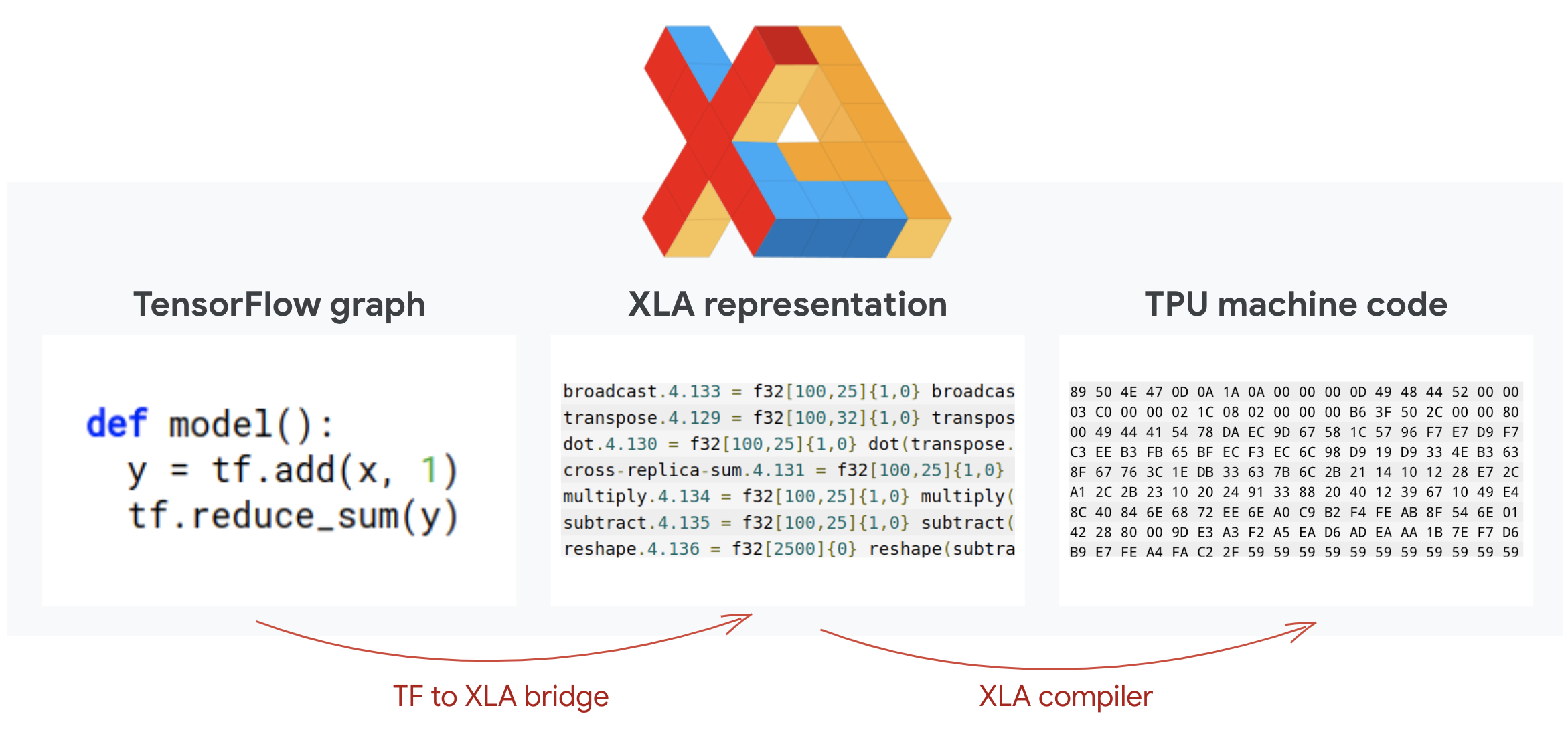
Illustration: to run on TPU, the computation graph defined by your Tensorflow program is first translated to an XLA (accelerated Linear Algebra compiler) representation, then compiled by XLA into TPU machine code.
Using TPUs in Keras
TPUs are supported through the Keras API as of Tensorflow 2.1. Keras support works on TPUs and TPU pods. Here is an example that works on TPU, GPU(s) and CPU:
try: # detect TPUs
    tpu = tf.distribute.cluster_resolver.TPUClusterResolver.connect()
    strategy = tf.distribute.TPUStrategy(tpu)
except ValueError: # detect GPUs
    strategy = tf.distribute.MirroredStrategy() # for CPU/GPU or multi-GPU machines

# use TPUStrategy scope to define model
with strategy.scope():
  model = tf.keras.Sequential( ... )
  model.compile( ... )

# train model normally on a tf.data.Dataset
model.fit(training_dataset, epochs=EPOCHS, steps_per_epoch=...)
In this code snippet:
TPUClusterResolver().connect()finds the TPU on the network. It works without parameters on most Google Cloud systems (AI Platform jobs, Colaboratory, Kubeflow, Deep Learning VMs created through the ‘ctpu up' utility). These systems know where their TPU is thanks to a TPU_NAME environment variable. If you create a TPU by hand, either set the TPU_NAME env. var. on the VM you are using it from, or callTPUClusterResolverwith explicit parameters:TPUClusterResolver(tp_uname, zone, project)TPUStrategyis the part that implements the distribution and the "all-reduce" gradient synchronization algorithm.- The strategy is applied through a scope. The model must be defined within the strategy scope().
- The
tpu_model.fitfunction expects a tf.data.Dataset object for input for TPU training.
Common TPU porting tasks
- While there are many ways to load data in a Tensorflow model, for TPUs, the use of the
tf.data.DatasetAPI is required. - TPUs are very fast and ingesting data often becomes the bottleneck when running on them. There are tools you can use to detect data bottlenecks and other performance tips in the TPU Performance Guide.
- int8 or int16 numbers are treated as int32. The TPU does not have integer hardware operating on less than 32 bits.
- Some Tensorflow operations are not supported. The list is here. The good news is that this limitation only applies to training code i.e. the forward and backward pass through your model. You can still use all Tensorflow operations in your data input pipeline as it will be executed on CPU.
tf.py_funcis not supported on TPU.
4. [INFO] Neural network classifier 101
In a nutshell
If all the terms in bold in the next paragraph are already known to you, you can move to the next exercise. If your are just starting in deep learning then welcome, and please read on.
For models built as a sequence of layers Keras offers the Sequential API. For example, an image classifier using three dense layers can be written in Keras as:
model = tf.keras.Sequential([
    tf.keras.layers.Flatten(input_shape=[192, 192, 3]),
    tf.keras.layers.Dense(500, activation="relu"),
    tf.keras.layers.Dense(50, activation="relu"),
    tf.keras.layers.Dense(5, activation='softmax') # classifying into 5 classes
])

# this configures the training of the model. Keras calls it "compiling" the model.
model.compile(
  optimizer='adam',
  loss= 'categorical_crossentropy',
  metrics=['accuracy']) # % of correct answers

# train the model
model.fit(dataset, ... )

Dense neural network
This is the simplest neural network for classifying images. It is made of "neurons" arranged in layers. The first layer processes input data and feeds its outputs into other layers. It is called "dense" because each neuron is connected to all the neurons in the previous layer.
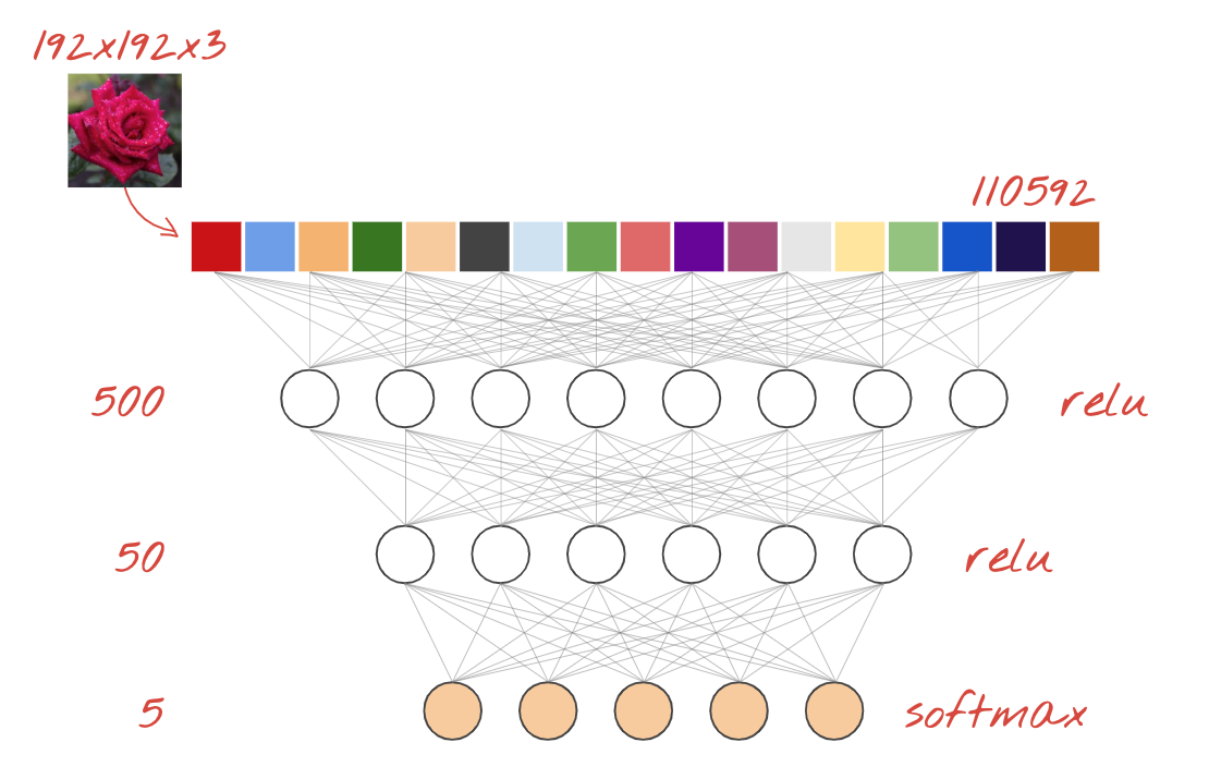
You can feed an image into such a network by flattening the RGB values of all of its pixels into a long vector and using it as inputs. It is not the best technique for image recognition but we will improve on it later.
Neurons, activations, RELU
A "neuron" computes a weighted sum of all of its inputs, adds a value called "bias" and feeds the result through a so called "activation function". The weights and bias are unknown at first. They will be initialized at random and "learned" by training the neural network on lots of known data.
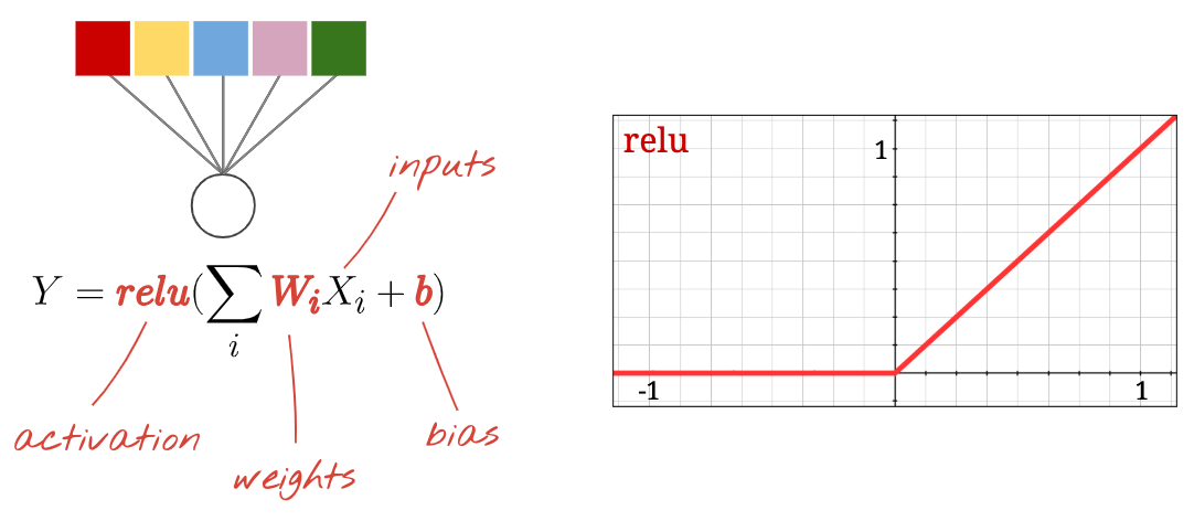
The most popular activation function is called RELU for Rectified Linear Unit. It is a very simple function as you can see on the graph above.
Softmax activation
The network above ends with a 5-neuron layer because we are classifying flowers into 5 categories (rose, tulip, dandelion, daisy, sunflower). Neurons in intermediate layers are activated using the classic RELU activation function. In the last layer though, we want to compute numbers between 0 and 1 representing the probability of this flower being a rose, a tulip and so on. For this, we will use an activation function called "softmax".
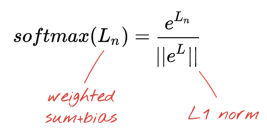
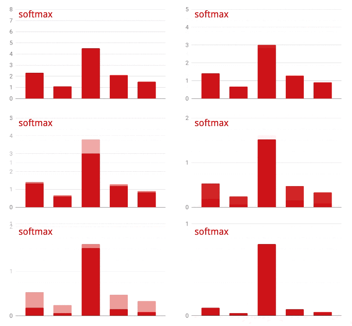
Applying softmax on a vector is done by taking the exponential of each element and then normalising the vector, typically using the L1 norm (sum of absolute values) so that the values add up to 1 and can be interpreted as probabilities.
Cross-entropy loss
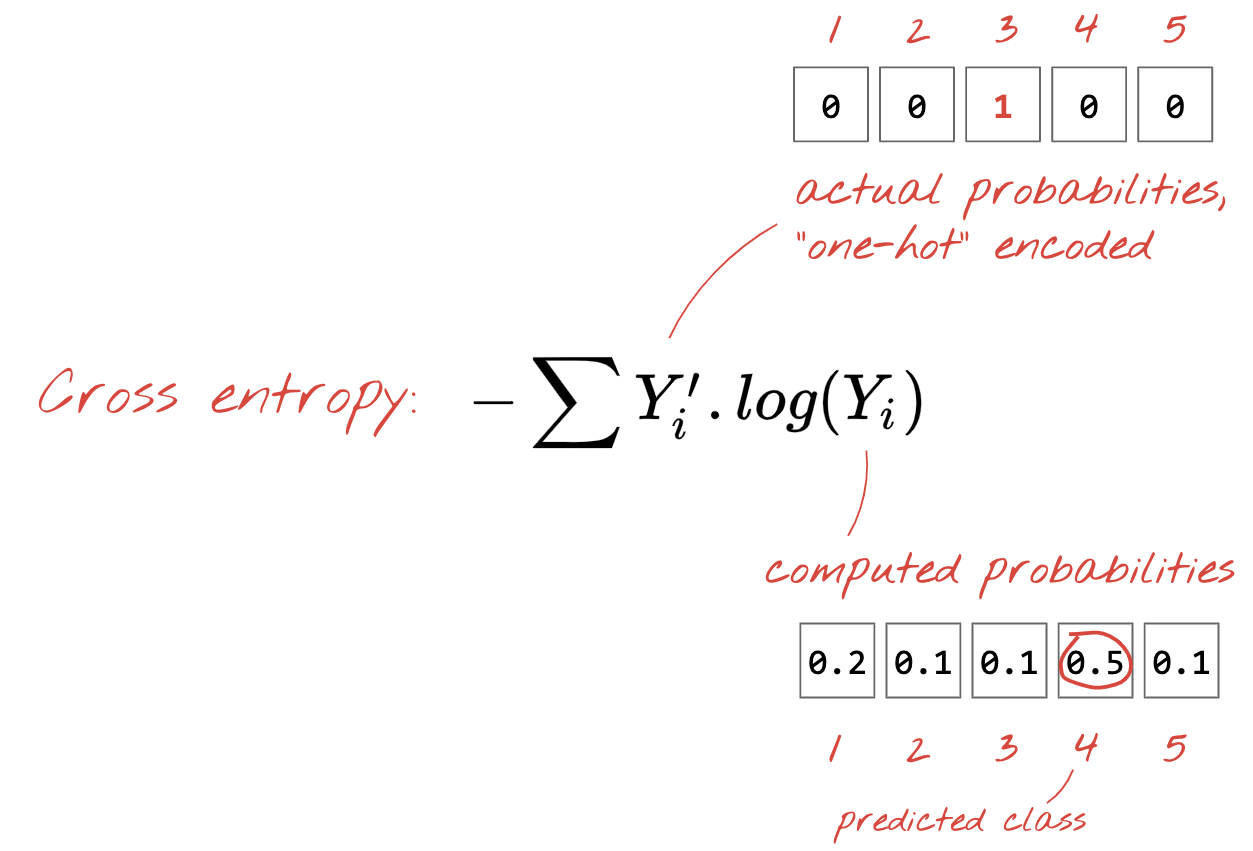
Now that our neural network produces predictions from input images, we need to measure how good they are, i.e. the distance between what the network tells us and the correct answers, often called "labels". Remember that we have correct labels for all the images in the dataset.
Any distance would work, but for classification problems the so-called "cross-entropy distance" is the most effective. We will call this our error or "loss" function:
Gradient descent
"Training" the neural network actually means using training images and labels to adjust weights and biases so as to minimise the cross-entropy loss function. Here is how it works.
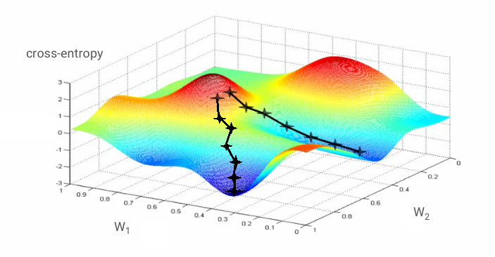
The cross-entropy is a function of weights, biases, pixels of the training image and its known class.
If we compute the partial derivatives of the cross-entropy relatively to all the weights and all the biases we obtain a "gradient", computed for a given image, label, and present value of weights and biases. Remember that we can have millions of weights and biases so computing the gradient sounds like a lot of work. Fortunately, Tensorflow does it for us. The mathematical property of a gradient is that it points "up". Since we want to go where the cross-entropy is low, we go in the opposite direction. We update weights and biases by a fraction of the gradient. We then do the same thing again and again using the next batches of training images and labels, in a training loop. Hopefully, this converges to a place where the cross-entropy is minimal although nothing guarantees that this minimum is unique.
Mini-batching and momentum
You can compute your gradient on just one example image and update the weights and biases immediately, but doing so on a batch of, for example, 128 images gives a gradient that better represents the constraints imposed by different example images and is therefore likely to converge towards the solution faster. The size of the mini-batch is an adjustable parameter.
This technique, sometimes called "stochastic gradient descent" has another, more pragmatic benefit: working with batches also means working with larger matrices and these are usually easier to optimise on GPUs and TPUs.
The convergence can still be a little chaotic though and it can even stop if the gradient vector is all zeros. Does that mean that we have found a minimum? Not always. A gradient component can be zero on a minimum or a maximum. With a gradient vector with millions of elements, if they are all zeros, the probability that every zero corresponds to a minimum and none of them to a maximum point is pretty small. In a space of many dimensions, saddle points are pretty common and we do not want to stop at them.
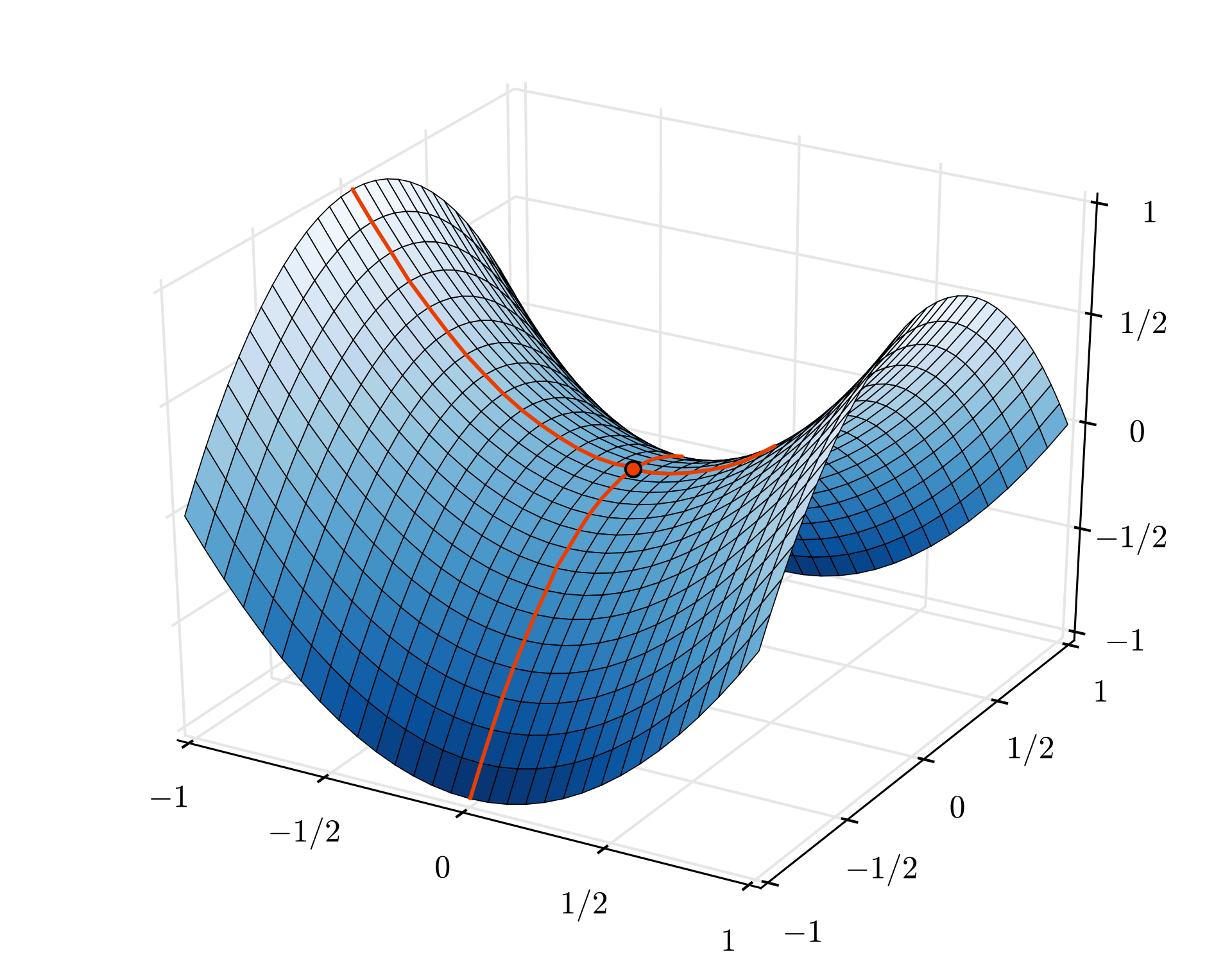
Illustration: a saddle point. The gradient is 0 but it is not a minimum in all directions. (Image attribution Wikimedia: By Nicoguaro - Own work, CC BY 3.0)
The solution is to add some momentum to the optimization algorithm so that it can sail past saddle points without stopping.
Glossary
batch or mini-batch: training is always performed on batches of training data and labels. Doing so helps the algorithm converge. The "batch" dimension is typically the first dimension of data tensors. For example a tensor of shape [100, 192, 192, 3] contains 100 images of 192x192 pixels with three values per pixel (RGB).
cross-entropy loss: a special loss function often used in classifiers.
dense layer: a layer of neurons where each neuron is connected to all the neurons in the previous layer.
features: the inputs of a neural network are sometimes called "features". The art of figuring out which parts of a dataset (or combinations of parts) to feed into a neural network to get good predictions is called "feature engineering".
labels: another name for "classes" or correct answers in a supervised classification problem
learning rate: fraction of the gradient by which weights and biases are updated at each iteration of the training loop.
logits: the outputs of a layer of neurons before the activation function is applied are called "logits". The term comes from the "logistic function" a.k.a. the "sigmoid function" which used to be the most popular activation function. "Neuron outputs before logistic function" was shortened to "logits".
loss: the error function comparing neural network outputs to the correct answers
neuron: computes the weighted sum of its inputs, adds a bias and feeds the result through an activation function.
one-hot encoding: class 3 out of 5 is encoded as a vector of 5 elements, all zeros except the 3rd one which is 1.
relu: rectified linear unit. A popular activation function for neurons.
sigmoid: another activation function that used to be popular and is still useful in special cases.
softmax: a special activation function that acts on a vector, increases the difference between the largest component and all others, and also normalizes the vector to have a sum of 1 so that it can be interpreted as a vector of probabilities. Used as the last step in classifiers.
tensor: A "tensor" is like a matrix but with an arbitrary number of dimensions. A 1-dimensional tensor is a vector. A 2-dimensions tensor is a matrix. And then you can have tensors with 3, 4, 5 or more dimensions.
5. [NEW INFO] Convolutional neural networks
In a nutshell
If all the terms in bold in the next paragraph are already known to you, you can move to the next exercise. If your are just starting with convolutional neural networks please read on.
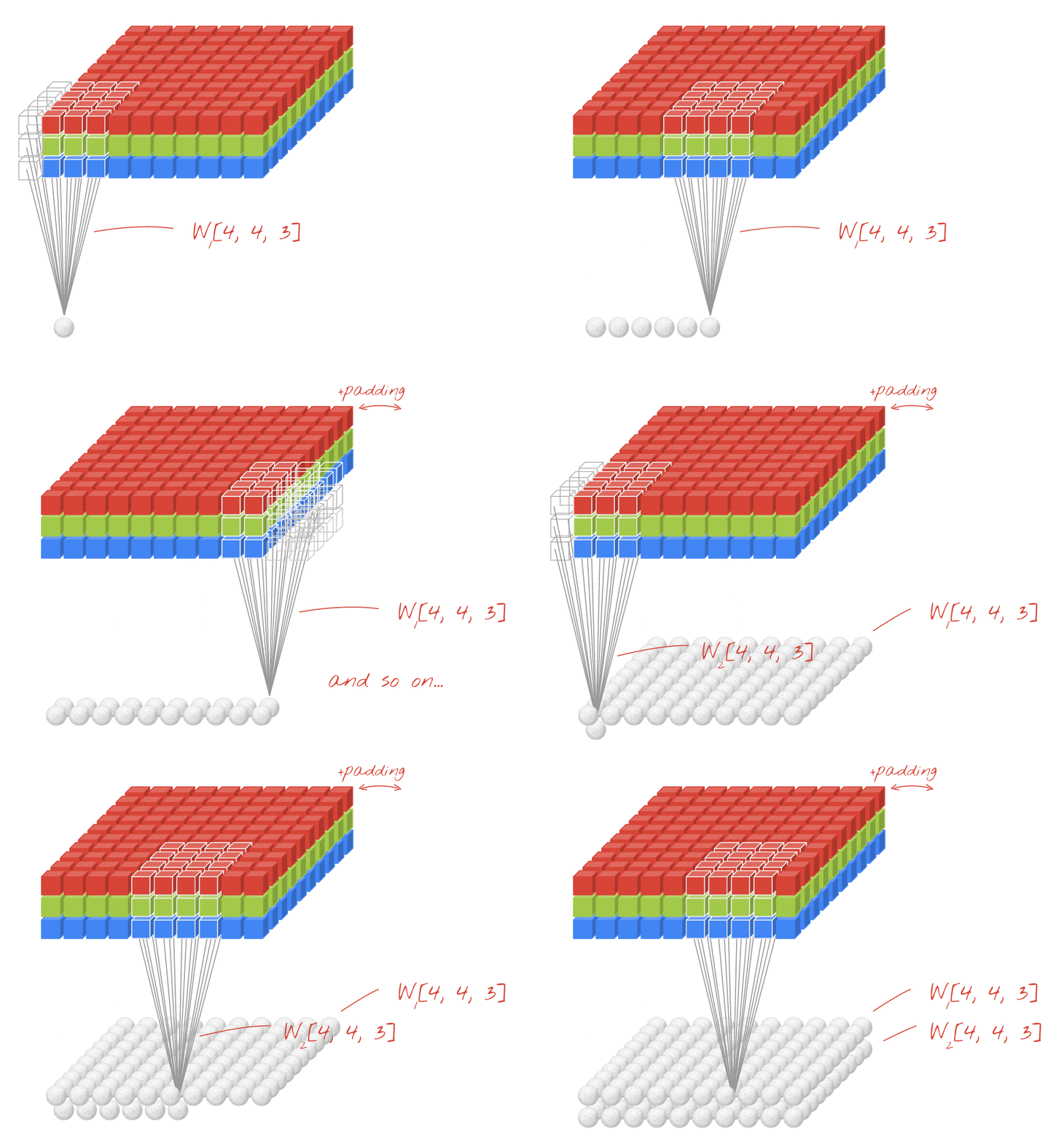
Illustration: filtering an image with two successive filters made of 4x4x3=48 learnable weights each.
This is how a simple convolutional neural network looks in Keras:
model = tf.keras.Sequential([
  # input: images of size 192x192x3 pixels (the three stands for RGB channels)
  tf.keras.layers.Conv2D(kernel_size=3, filters=24, padding='same', activation='relu', input_shape=[192, 192, 3]),
  tf.keras.layers.Conv2D(kernel_size=3, filters=24, padding='same', activation='relu'),
  tf.keras.layers.MaxPooling2D(pool_size=2),
  tf.keras.layers.Conv2D(kernel_size=3, filters=12, padding='same', activation='relu'),
  tf.keras.layers.MaxPooling2D(pool_size=2),
  tf.keras.layers.Conv2D(kernel_size=3, filters=6, padding='same', activation='relu'),
  tf.keras.layers.Flatten(),
  # classifying into 5 categories
  tf.keras.layers.Dense(5, activation='softmax')
])

model.compile(
  optimizer='adam',
  loss= 'categorical_crossentropy',
  metrics=['accuracy'])

Convolutional neural nets 101
In a layer of a convolutional network, one "neuron" does a weighted sum of the pixels just above it, across a small region of the image only. It adds a bias and feeds the sum through an activation function, just as a neuron in a regular dense layer would. This operation is then repeated across the entire image using the same weights. Remember that in dense layers, each neuron had its own weights. Here, a single "patch" of weights slides across the image in both directions (a "convolution"). The output has as many values as there are pixels in the image (some padding is necessary at the edges though). It is a filtering operation, using a filter of 4x4x3=48 weights.
However, 48 weights will not be enough. To add more degrees of freedom, we repeat the same operation with a new set of weights. This produces a new set of filter outputs. Let's call it a "channel" of outputs by analogy with the R,G,B channels in the input image.
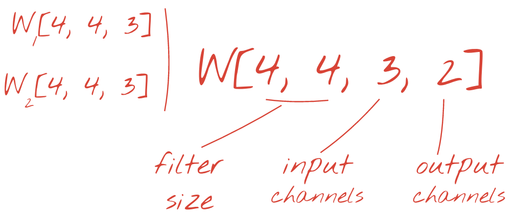
The two (or more) sets of weights can be summed up as one tensor by adding a new dimension. This gives us the generic shape of the weights tensor for a convolutional layer. Since the number of input and output channels are parameters, we can start stacking and chaining convolutional layers.
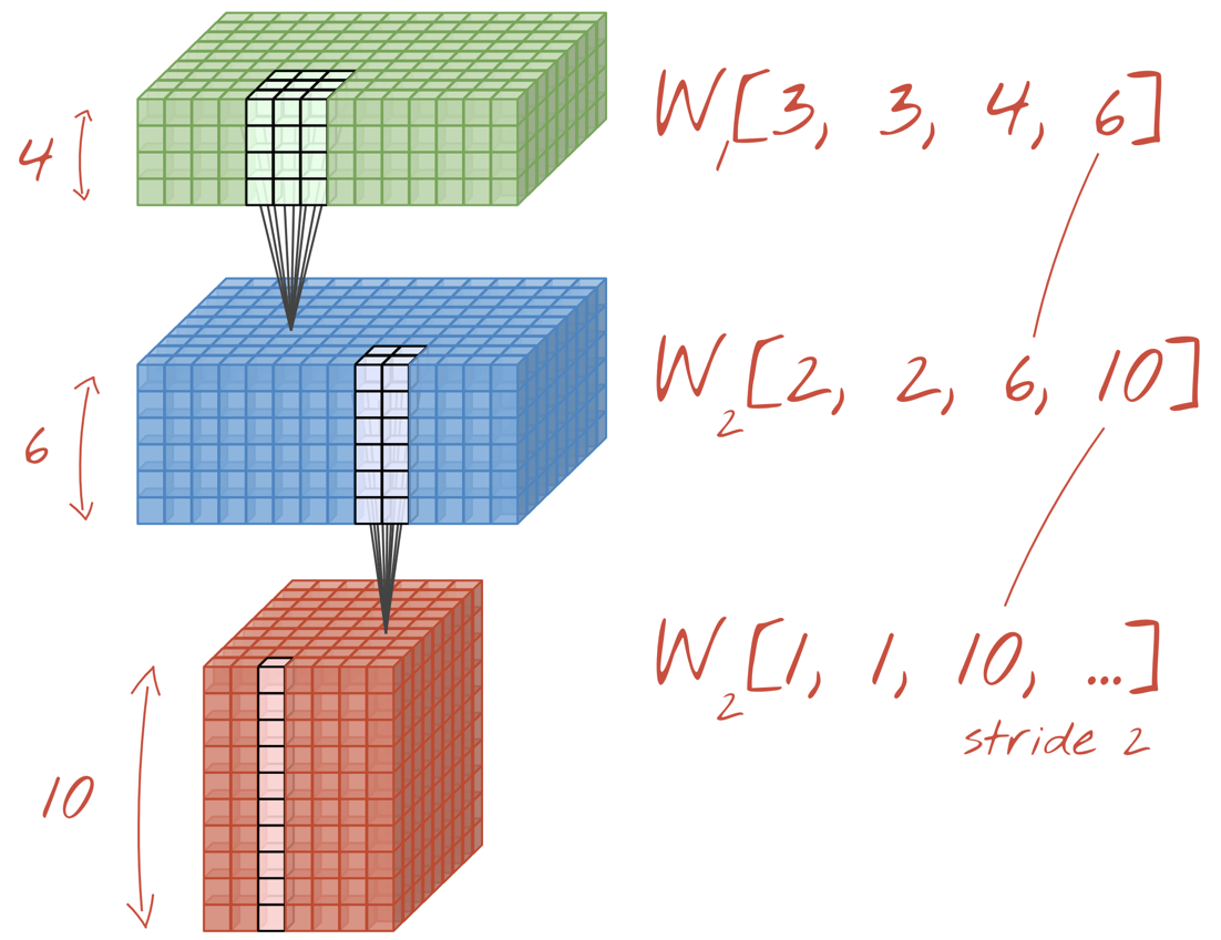
Illustration: a convolutional neural network transforms "cubes" of data into other "cubes" of data.
Strided convolutions, max pooling
By performing the convolutions with a stride of 2 or 3, we can also shrink the resulting data cube in its horizontal dimensions. There are two common ways of doing this:
- Strided convolution: a sliding filter as above but with a stride >1
- Max pooling: a sliding window applying the MAX operation (typically on 2x2 patches, repeated every 2 pixels)
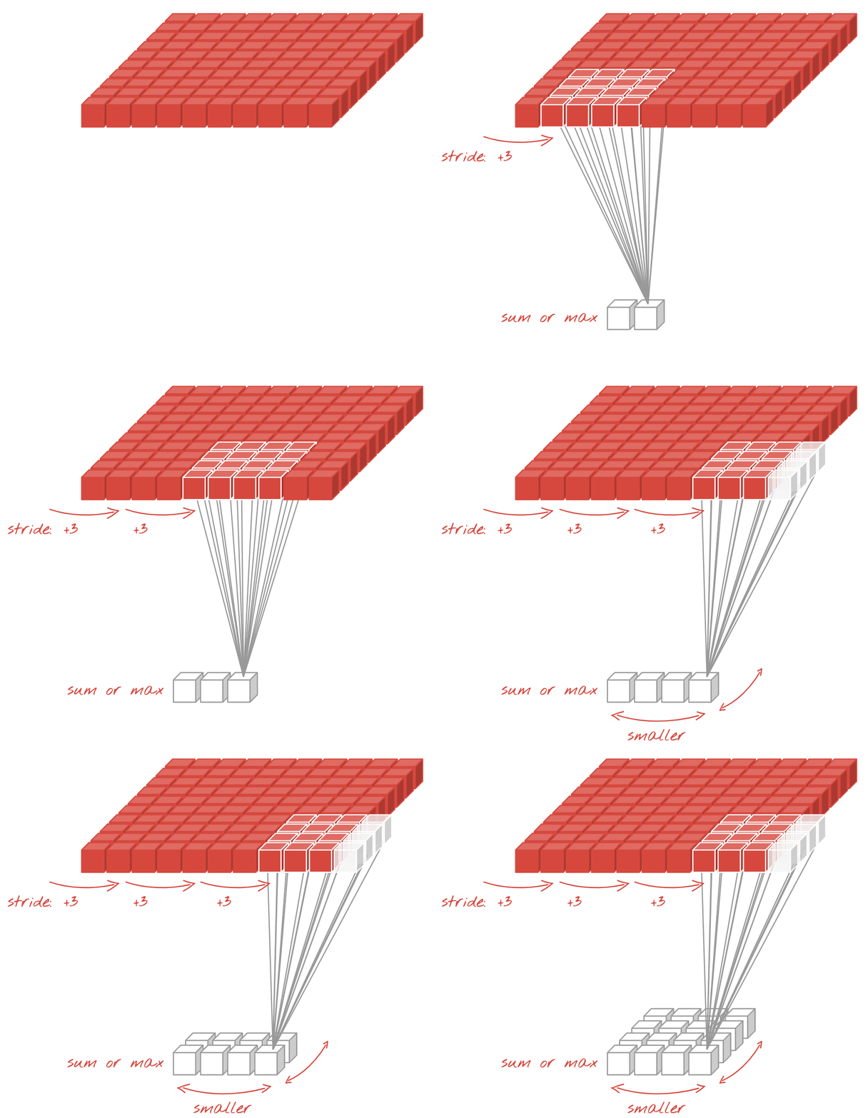
Illustration: sliding the computing window by 3 pixels results in fewer output values. Strided convolutions or max pooling (max on a 2x2 window sliding by a stride of 2) are a way of shrinking the data cube in the horizontal dimensions.
Convolutional classifier
Finally, we attach a classification head by flattening the last data cube and feeding it through a dense, softmax-activated layer. A typical convolutional classifier can look like this:
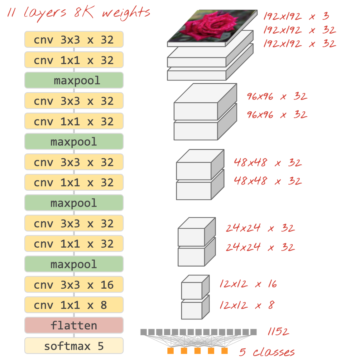
Illustration: an image classifier using convolutional and softmax layers. It uses 3x3 and 1x1 filters. The maxpool layers take the max of groups of 2x2 data points. The classification head is implemented with a dense layer with softmax activation.
In Keras
The convolutional stack illustrated above can be written in Keras like this:
model = tf.keras.Sequential([
  # input: images of size 192x192x3 pixels (the three stands for RGB channels)
  tf.keras.layers.Conv2D(kernel_size=3, filters=32, padding='same', activation='relu', input_shape=[192, 192, 3]),
  tf.keras.layers.Conv2D(kernel_size=1, filters=32, padding='same', activation='relu'),
  tf.keras.layers.MaxPooling2D(pool_size=2),
  tf.keras.layers.Conv2D(kernel_size=3, filters=32, padding='same', activation='relu'),
  tf.keras.layers.Conv2D(kernel_size=1, filters=32, padding='same', activation='relu'),
  tf.keras.layers.MaxPooling2D(pool_size=2),
  tf.keras.layers.Conv2D(kernel_size=3, filters=32, padding='same', activation='relu'),
  tf.keras.layers.Conv2D(kernel_size=1, filters=32, padding='same', activation='relu'),
  tf.keras.layers.MaxPooling2D(pool_size=2),
  tf.keras.layers.Conv2D(kernel_size=3, filters=32, padding='same', activation='relu'),
  tf.keras.layers.Conv2D(kernel_size=1, filters=32, padding='same', activation='relu'),
  tf.keras.layers.MaxPooling2D(pool_size=2),
  tf.keras.layers.Conv2D(kernel_size=3, filters=16, padding='same', activation='relu'),
  tf.keras.layers.Conv2D(kernel_size=1, filters=8, padding='same', activation='relu'),
  tf.keras.layers.Flatten(),
  # classifying into 5 categories
  tf.keras.layers.Dense(5, activation='softmax')
])

model.compile(
  optimizer='adam',
  loss= 'categorical_crossentropy',
  metrics=['accuracy'])
6. Your custom convnet
Hands-on
Let us build and train a convolutional neural network from scratch. Using a TPU will allow us to iterate very fast. Please open the following notebook, execute the cells (Shift-ENTER) and follow the instructions wherever you see a "WORK REQUIRED" label.

Keras_Flowers_TPU (playground).ipynb
The goal is to beat the 75% accuracy of the transfer learning model. That model had an advantage, having been pre-trained on a dataset of millions of images while we only have 3670 images here. Can you at least match it?
Additional information
How many layers, how big?
Selecting layer sizes is more of an art than a science. You have to find the right balance between having too few and too many parameters (weights and biases). With too few weights, the neural network cannot represent the complexity of flower shapes. With too many, it can be prone to "overfitting", i.e. specializing in the training images and not being able to generalize. With a lot of parameters, the model will also be slow to train. In Keras, the model.summary() function displays the structure and parameter count of your model:
Layer (type)                 Output Shape              Param #
=================================================================
conv2d (Conv2D)              (None, 192, 192, 16)      448
_________________________________________________________________
conv2d_1 (Conv2D)            (None, 192, 192, 30)      4350
_________________________________________________________________
max_pooling2d (MaxPooling2D) (None, 96, 96, 30)        0
_________________________________________________________________
conv2d_2 (Conv2D)            (None, 96, 96, 60)        16260
_________________________________________________________________
 ...
_________________________________________________________________
global_average_pooling2d (Gl (None, 130)               0
_________________________________________________________________
dense (Dense)                (None, 90)                11790
_________________________________________________________________
dense_1 (Dense)              (None, 5)                 455
=================================================================
Total params: 300,033
Trainable params: 300,033
Non-trainable params: 0
_________________________________________________________________
A couple of tips:
- Having multiple layers is what makes "deep" neural networks effective. For this simple flower recognition problem, 5 to 10 layers make sense.
- Use small filters. Typically 3x3 filters are good everywhere.
- 1x1 filters can be used too and are cheap. They do not really "filter" anything but compute linear combinations of channels. Alternate them with real filters. (More about "1x1 convolutions" in the next section.)
- For a classification problem like this, downsample frequently with max-pooling layers (or convolutions with stride >1). You do not care where the flower is, only that it is a rose or a dandelion so losing x and y information is not important and filtering smaller areas is cheaper.
- The number of filters usually becomes similar to the number of classes at the end of the network (why? see "global average pooling" trick below). If you classify into hundreds of classes, increase the filter count progressively in consecutive layers. For the flower dataset with 5 classes, filtering with only 5 filters would not be enough. You can use the same filter count in most layers, for example 32 and decrease it towards the end.
- The final dense layer(s) is/are expensive. It/they can have more weights than all the convolutional layers combined. For example, even with a very reasonable output from the last data cube of 24x24x10 data points, a 100 neuron dense layer would cost 24x24x10x100=576,000 weights !!! Try to be thoughtful, or try global average pooling (see below).
Global average pooling
Instead of using an expensive dense layer at the end of a convolutional neural network, you can split the incoming data "cube" into as many parts as you have classes, average their values and feed these through a softmax activation function. This way of building the classification head costs 0 weights. In Keras, the syntax is tf.keras.layers.GlobalAveragePooling2D().
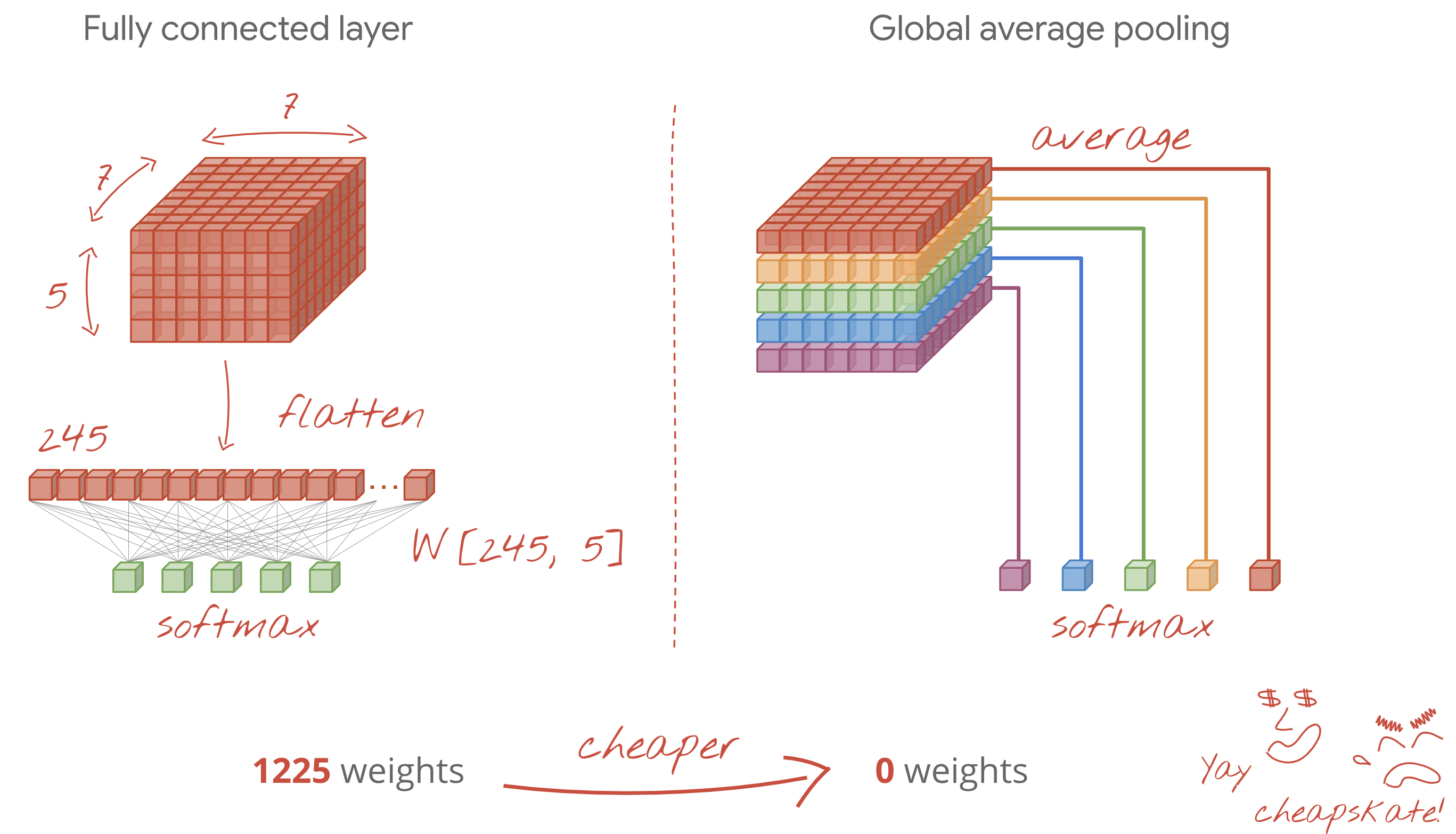
Solution
Here is the solution notebook. You can use it if you are stuck.

Keras_Flowers_TPU (solution).ipynb
What we've covered
- 🤔 Played with convolutional layers
- 🤓 Experimented with max pooling, strides, global average pooling, ...
- 😀 iterated on a real-world model fast, on TPU
Please take a moment to go through this checklist in your head.
7. Congratulations!
You have built your first modern convolutional neural network and trained it to 80% + accuracy, iterating on its architecture in only minutes thanks to TPUs. Please continue to the next lab to learn about modern convolutional architectures:
- TPU-speed data pipelines: tf.data.Dataset and TFRecords
- Your first Keras model, with transfer learning
- [THIS LAB] Convolutional neural networks, with Keras and TPUs
- Modern convnets, squeezenet, Xception, with Keras and TPUs
TPUs in practice
TPUs and GPUs are available on Cloud AI Platform:
- On Deep Learning VMs
- In AI Platform Notebooks
- In AI Platform Training jobs
Finally, we love feedback. Please tell us if you see something amiss in this lab or if you think it should be improved. Feedback can be provided through GitHub issues [ feedback link].

|


