
১. ভূমিকা
সর্বশেষ হালনাগাদ: ২০২১-০৯-১৫
মূল্য নির্ধারণ সংক্রান্ত অন্তর্দৃষ্টি এবং অপ্টিমাইজেশনের জন্য প্রয়োজনীয় ডেটা স্বভাবতই ভিন্ন ভিন্ন প্রকৃতির হয় (যেমন ভিন্ন সিস্টেম, ভিন্ন স্থানীয় বাস্তবতা ইত্যাদি), তাই একটি সুগঠিত, মানসম্মত এবং ত্রুটিমুক্ত সিডিএম (CDM) টেবিল তৈরি করা অত্যন্ত গুরুত্বপূর্ণ। এর মধ্যে মূল্য নির্ধারণ অপ্টিমাইজেশনের জন্য লেনদেন, পণ্য, মূল্য এবং গ্রাহকের মতো মূল বৈশিষ্ট্যগুলো অন্তর্ভুক্ত থাকে। এই ডকুমেন্টে, আমরা আপনাকে নিচে বর্ণিত ধাপগুলো ধাপে ধাপে দেখিয়ে দেব, যা প্রাইসিং অ্যানালিটিক্সের জন্য একটি দ্রুত সূচনা প্রদান করবে এবং আপনি এটিকে আপনার নিজের প্রয়োজন অনুযায়ী প্রসারিত ও কাস্টমাইজ করতে পারবেন। নিম্নলিখিত ডায়াগ্রামটি এই ডকুমেন্টে আলোচিত ধাপগুলো তুলে ধরেছে।
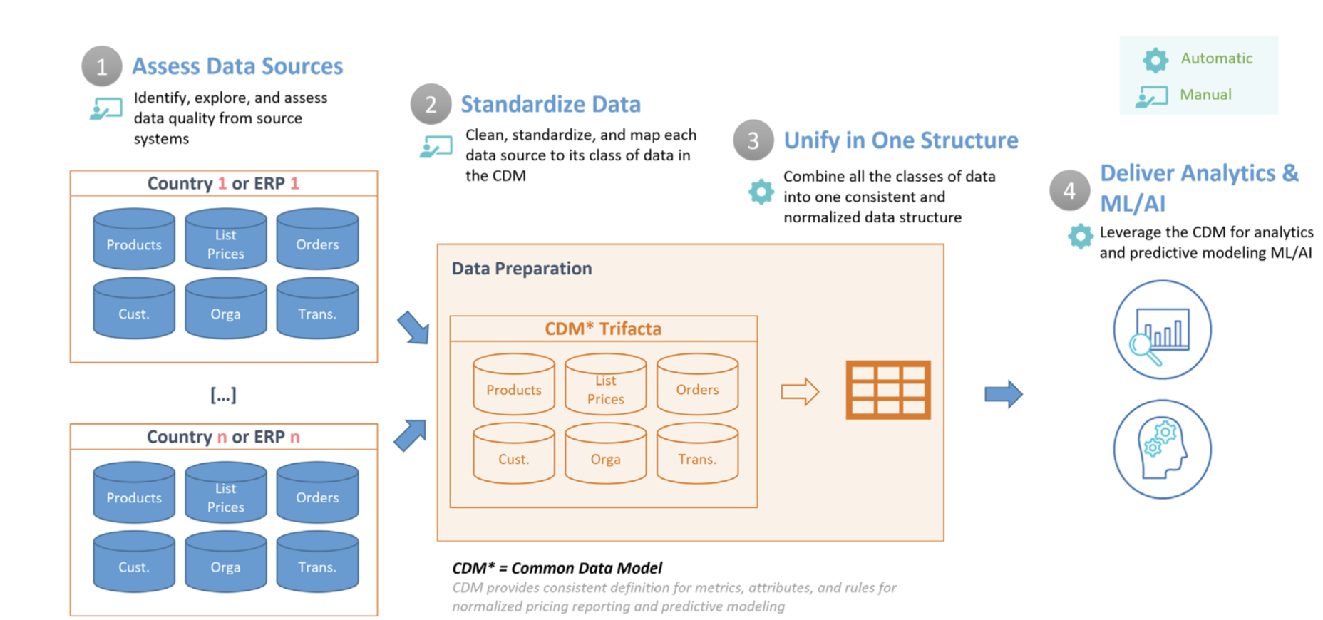
- ডেটা উৎস মূল্যায়ন করুন: প্রথমে, আপনাকে সেই ডেটা উৎসগুলোর একটি তালিকা তৈরি করতে হবে যা সিডিএম (CDM) তৈরি করতে ব্যবহৃত হবে। এই ধাপে, ইনপুট ডেটা থেকে সমস্যাগুলো খুঁজে বের করতে ও শনাক্ত করতে ডেটাপ্রেপ (Dataprep) ব্যবহার করা হয়। উদাহরণস্বরূপ, অনুপস্থিত ও অমিল মান, নামকরণের অসঙ্গতি, ডুপ্লিকেট, ডেটার অখণ্ডতার সমস্যা, আউটলায়ার ইত্যাদি।
- ডেটা মানসম্মতকরণ: এরপর, ডেটার নির্ভুলতা, অখণ্ডতা, সামঞ্জস্য এবং সম্পূর্ণতা নিশ্চিত করার জন্য পূর্বে চিহ্নিত সমস্যাগুলো সমাধান করা হয়। এই প্রক্রিয়ায় ডেটাপ্রেপ (Dataprep)-এ বিভিন্ন রূপান্তর অন্তর্ভুক্ত থাকতে পারে, যেমন তারিখের ফরম্যাটিং, মানের মানসম্মতকরণ, একক রূপান্তর, অপ্রয়োজনীয় ফিল্ড ও মান ফিল্টার করে বাদ দেওয়া এবং উৎস ডেটাকে বিভক্ত করা, যুক্ত করা বা ডুপ্লিকেট ডেটা অপসারণ করা।
- একটি কাঠামোতে একীভূত করুন: পাইপলাইনের পরবর্তী ধাপে প্রতিটি ডেটা সোর্সকে BigQuery- তে একটি একক, প্রশস্ত টেবিলে যুক্ত করা হয়, যেখানে সূক্ষ্মতম স্তরের সমস্ত অ্যাট্রিবিউট অন্তর্ভুক্ত থাকে। এই ডিনরমালাইজড কাঠামোটি এমন কার্যকর অ্যানালিটিক্যাল কোয়েরির সুযোগ করে দেয়, যেগুলোর জন্য জয়েনের প্রয়োজন হয় না।
- অ্যানালিটিক্স ও এমএল/এআই সরবরাহ করুন: ডেটা একবার বিশ্লেষণের জন্য পরিষ্কার এবং ফরম্যাট করা হয়ে গেলে, বিশ্লেষকরা পূর্ববর্তী মূল্য পরিবর্তনের প্রভাব বোঝার জন্য ঐতিহাসিক ডেটা খতিয়ে দেখতে পারেন। এছাড়াও, ভবিষ্যতের বিক্রয় অনুমান করার জন্য প্রেডিক্টিভ মডেল তৈরি করতে BigQuery ML ব্যবহার করা যেতে পারে। এই মডেলগুলির আউটপুট Looker- এর ড্যাশবোর্ডে অন্তর্ভুক্ত করে "হোয়াট-ইফ সিনারিও" তৈরি করা যায়, যেখানে ব্যবসায়িক ব্যবহারকারীরা বিশ্লেষণ করতে পারেন যে নির্দিষ্ট মূল্য পরিবর্তনের ফলে বিক্রয় কেমন হতে পারে।
নিম্নলিখিত ডায়াগ্রামটি প্রাইসিং অপটিমাইজেশন অ্যানালিটিক্স পাইপলাইন তৈরি করতে ব্যবহৃত গুগল ক্লাউড উপাদানগুলো দেখায়।

আপনি যা তৈরি করবেন
এখানে আমরা আপনাকে দেখাবো কিভাবে একটি প্রাইসিং অপটিমাইজেশন ডেটা ওয়্যারহাউস ডিজাইন করতে হয়, সময়ের সাথে সাথে ডেটা প্রস্তুতির প্রক্রিয়াকে স্বয়ংক্রিয় করতে হয়, পণ্যের মূল্যের পরিবর্তনের প্রভাব অনুমান করতে মেশিন লার্নিং ব্যবহার করতে হয় এবং আপনার টিমকে কার্যকরী অন্তর্দৃষ্টি প্রদানের জন্য রিপোর্ট তৈরি করতে হয়।
আপনি যা শিখবেন
- প্রাইসিং অ্যানালিটিক্সের জন্য ডেটাপ্রেপকে কীভাবে ডেটা সোর্সের সাথে সংযুক্ত করবেন, যা রিলেশনাল ডেটাবেস, ফ্ল্যাট ফাইল, গুগল শিটস এবং অন্যান্য সমর্থিত অ্যাপ্লিকেশনে সংরক্ষিত থাকতে পারে।
- আপনার BigQuery ডেটা ওয়্যারহাউসে একটি CDM টেবিল তৈরি করার জন্য কীভাবে একটি Dataprep ফ্লো তৈরি করবেন।
- ভবিষ্যৎ রাজস্বের পূর্বাভাস দিতে BigQuery ML কীভাবে ব্যবহার করবেন।
- ঐতিহাসিক মূল্য নির্ধারণ ও বিক্রয়ের প্রবণতা বিশ্লেষণ করতে এবং ভবিষ্যতের মূল্য পরিবর্তনের প্রভাব বুঝতে Looker- এ কীভাবে রিপোর্ট তৈরি করবেন।
আপনার যা যা লাগবে
- বিলিং চালু থাকা একটি গুগল ক্লাউড প্রজেক্ট। আপনার প্রজেক্টের জন্য বিলিং চালু আছে কিনা, তা কীভাবে নিশ্চিত করবেন তা জানুন ।
- আপনার প্রোজেক্টে BigQuery অবশ্যই সক্রিয় করতে হবে। নতুন প্রোজেক্টে এটি স্বয়ংক্রিয়ভাবে সক্রিয় হয়ে যায়। অন্যথায়, বিদ্যমান কোনো প্রোজেক্টে এটি সক্রিয় করুন । এছাড়া, আপনি এখান থেকে ক্লাউড কনসোলের মাধ্যমে BigQuery ব্যবহার শুরু করার বিষয়ে আরও জানতে পারেন।
- আপনার প্রোজেক্টে ডেটাপ্রেপও অবশ্যই সক্রিয় করতে হবে। গুগল কনসোলের বাম দিকের নেভিগেশন মেনুর বিগ ডেটা সেকশন থেকে ডেটাপ্রেপ সক্রিয় করা হয়। এটি সক্রিয় করতে সাইন আপের ধাপগুলো অনুসরণ করুন।
- আপনার নিজস্ব Looker ড্যাশবোর্ড সেট আপ করার জন্য, একটি Looker ইনস্ট্যান্সে আপনার ডেভেলপার অ্যাক্সেস থাকতে হবে। ট্রায়ালের জন্য অনুরোধ করতে অনুগ্রহ করে এখানে আমাদের টিমের সাথে যোগাযোগ করুন , অথবা আমাদের নমুনা ডেটার উপর ডেটা পাইপলাইনের ফলাফলগুলি অন্বেষণ করতে আমাদের পাবলিক ড্যাশবোর্ড ব্যবহার করুন।
- স্ট্রাকচার্ড কোয়েরি ল্যাঙ্গুয়েজ (SQL)-এর অভিজ্ঞতা এবং নিম্নলিখিত বিষয়গুলো সম্পর্কে প্রাথমিক জ্ঞান থাকলে সহায়ক হবে: ট্রাইফ্যাক্টার ডেটাপ্রেপ (Dataprep by Trifacta) , বিগকোয়েরি (BigQuery) , লুকার (Looker)।
২. BigQuery-তে CDM তৈরি করুন
এই অংশে, আপনি কমন ডেটা মডেল (CDM) তৈরি করেন, যা মূল্য নির্ধারণে পরিবর্তন বিশ্লেষণ ও পরামর্শ দেওয়ার জন্য প্রয়োজনীয় তথ্যের একটি সমন্বিত চিত্র প্রদান করে।
- BigQuery কনসোলটি খুলুন।
- এই রেফারেন্স প্যাটার্নটি পরীক্ষা করার জন্য আপনি যে প্রজেক্টটি ব্যবহার করতে চান, সেটি নির্বাচন করুন।
- বিদ্যমান কোনো ডেটাসেট ব্যবহার করুন অথবা একটি BigQuery ডেটাসেট তৈরি করুন । ডেটাসেটটির নাম দিন
Pricing_CDM। - টেবিলটি তৈরি করুন :
create table `CDM_Pricing`
(
  Fiscal_Date DATETIME,
  Product_ID STRING,
  Client_ID INT64,
  Customer_Hierarchy STRING,
  Division STRING,
  Market STRING,
  Channel STRING,
  Customer_code INT64,
  Customer_Long_Description STRING,
  Key_Account_Manager INT64,
  Key_Account_Manager_Description STRING,
  Structure STRING,
  Invoiced_quantity_in_Pieces FLOAT64,
  Gross_Sales FLOAT64,
  Trade_Budget_Costs FLOAT64,
  Cash_Discounts_and_other_Sales_Deductions INT64,
  Net_Sales FLOAT64,
  Variable_Production_Costs_STD FLOAT64,
  Fixed_Production_Costs_STD FLOAT64,
  Other_Cost_of_Sales INT64,
  Standard_Gross_Margin FLOAT64,
  Transportation_STD FLOAT64,
  Warehouse_STD FLOAT64,
  Gross_Margin_After_Logistics FLOAT64,
  List_Price_Converged FLOAT64
);
৩. তথ্যের উৎস মূল্যায়ন করুন
এই টিউটোরিয়ালে, আপনি গুগল শিটস এবং বিগকোয়েরি- তে সংরক্ষিত নমুনা ডেটা সোর্স ব্যবহার করবেন।
- লেনদেন সংক্রান্ত গুগল শিটটিতে প্রতিটি লেনদেনের জন্য একটি করে সারি রয়েছে। এতে বিক্রি হওয়া প্রতিটি পণ্যের পরিমাণ, মোট স্থূল বিক্রয় এবং সংশ্লিষ্ট খরচের মতো বিবরণ রয়েছে।
- পণ্যের মূল্য নির্ধারণ সংক্রান্ত গুগল শিট, যেখানে একজন নির্দিষ্ট গ্রাহকের জন্য প্রতি মাসের প্রতিটি পণ্যের মূল্য উল্লেখ থাকে।
- `company_descriptions` BigQuery টেবিলটিতে স্বতন্ত্র গ্রাহকদের তথ্য থাকে।
নিম্নলিখিত স্টেটমেন্টটি ব্যবহার করে এই `company_descriptions` BigQuery টেবিলটি তৈরি করা যায়:
create table `Company_Descriptions`
(
 Customer_ID INT64,
 Customer_Long_Description STRING
);
insert into `Company_Descriptions` values (15458, 'ENELTEN');
insert into `Company_Descriptions` values (16080, 'NEW DEVICES CORP.');
insert into `Company_Descriptions` values (19913, 'ENELTENGAS');
insert into `Company_Descriptions` values (30108, 'CARTOON NT');
insert into `Company_Descriptions` values (32492, 'Thomas Ed Automobiles');
৪. প্রবাহ তৈরি করুন
এই ধাপে, আপনি একটি নমুনা ডেটাপ্রেপ ফ্লো ইম্পোর্ট করবেন, যা পূর্ববর্তী বিভাগে তালিকাভুক্ত উদাহরণ ডেটাসেটগুলোকে রূপান্তর ও একীভূত করতে ব্যবহৃত হয়। একটি ফ্লো হলো একটি পাইপলাইন বা অবজেক্ট, যা ডেটাসেট এবং রেসিপিগুলোকে একত্রিত করে, যেগুলো সেগুলোকে রূপান্তর ও সংযুক্ত করতে ব্যবহৃত হয়।
- গিটহাব থেকে প্রাইসিং অপটিমাইজেশন প্যাটার্ন ফ্লো প্যাকেজটি ডাউনলোড করুন, কিন্তু এটি আনজিপ করবেন না। এই ফাইলটিতে প্রাইসিং অপটিমাইজেশন ডিজাইন প্যাটার্ন ফ্লো রয়েছে, যা স্যাম্পল ডেটা রূপান্তর করতে ব্যবহৃত হয়।
- Dataprep-এ, বাম দিকের নেভিগেশন বারে থাকা Flows আইকনে ক্লিক করুন। এরপর Flows ভিউতে, কনটেক্সট মেনু থেকে Import নির্বাচন করুন। ফ্লোটি ইম্পোর্ট করার পর, আপনি সেটি দেখতে ও সম্পাদনা করতে নির্বাচন করতে পারেন।

- ফ্লো-এর বাম দিকে, প্রোডাক্ট প্রাইসিং এবং তিনটি ট্রানজ্যাকশন গুগল শিটস-এর প্রত্যেকটিকে ডেটাসেট হিসেবে সংযুক্ত করতে হবে। এটি করার জন্য, গুগল শিটস ডেটাসেট অবজেক্টগুলোর উপর রাইট-ক্লিক করুন এবং রিপ্লেস (Replace ) নির্বাচন করুন। এরপর ইমপোর্ট ডেটাসেটস (Import Datasets) লিঙ্কে ক্লিক করুন। নিচের ডায়াগ্রামে দেখানো অনুযায়ী, "এডিট পাথ" (Edit path) পেন্সিল আইকনে ক্লিক করুন।
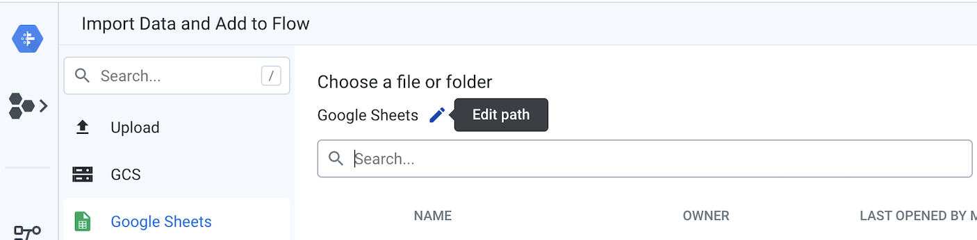
বর্তমান মানটিকে লেনদেন এবং পণ্যের মূল্য নির্ধারণ সম্পর্কিত গুগল শিটস-এর লিঙ্ক দিয়ে প্রতিস্থাপন করুন ।
যখন গুগল শিটসে একাধিক ট্যাব থাকে, তখন আপনি মেনু থেকে আপনার পছন্দের ট্যাবটি বেছে নিতে পারেন। এডিট (Edit)- এ ক্লিক করুন এবং ডেটা সোর্স হিসেবে ব্যবহার করতে চান এমন ট্যাবগুলো নির্বাচন করুন, তারপর সেভ (Save)- এ ক্লিক করুন এবং ইমপোর্ট অ্যান্ড অ্যাড টু ফ্লো (Import & Add to Flow)- তে ক্লিক করুন। যখন আপনি মডালে ফিরে আসবেন, তখন রিপ্লেস (Replace)- এ ক্লিক করুন। এই ফ্লো-তে, প্রতিটি শীটকে তার নিজস্ব ডেটাসেট হিসেবে দেখানো হয়েছে, যাতে পরবর্তী একটি রেসিপিতে বিভিন্ন সোর্সকে একত্রিত করার পদ্ধতি প্রদর্শন করা যায়।

- BigQuery আউটপুট টেবিলগুলি সংজ্ঞায়িত করুন:
এই ধাপে, আপনি BigQuery CDM_Pricing আউটপুট টেবিলের অবস্থানটি নির্ধারণ করবেন, যাতে প্রতিবার Dataoprep জব চালানোর সময় এটি লোড হয়।
ফ্লো ভিউ-তে, স্কিমা ম্যাপিং আউটপুট আইকনে ক্লিক করুন, ডিটেইলস প্যানেলে, ডেস্টিনেশনস ট্যাবে ক্লিক করুন। সেখান থেকে, পরীক্ষার জন্য ব্যবহৃত ম্যানুয়াল ডেস্টিনেশনস আউটপুট এবং যখন আপনি আপনার সম্পূর্ণ ফ্লো স্বয়ংক্রিয় করতে চান তখন ব্যবহৃত শিডিউলড ডেস্টিনেশনস আউটপুট উভয়ই সম্পাদনা করুন। এটি করার জন্য এই নির্দেশাবলী অনুসরণ করুন:
- ডিটেইলস প্যানেলে, ম্যানুয়াল ডেস্টিনেশনস সেকশনের অধীনে, এডিট বাটনে ক্লিক করুন। পাবলিশিং সেটিংস পেজে, পাবলিশিং অ্যাকশনস-এর অধীনে, যদি কোনো পাবলিশিং অ্যাকশন আগে থেকেই থাকে, তবে সেটি এডিট করুন, অন্যথায় অ্যাড অ্যাকশন বাটনে ক্লিক করুন। সেখান থেকে, BigQuery ডেটাসেট ব্যবহার করে পূর্ববর্তী ধাপে তৈরি করা
Pricing_CDMডেটাসেটে যান এবংCDM_Pricingটেবিলটি সিলেক্ট করুন। নিশ্চিত করুন যে ‘Append to this table every run’ অপশনটি চেক করা আছে এবং তারপর অ্যাড -এ ক্লিক করুন। সেভ সেটিংস-এ ক্লিক করুন। - "নির্ধারিত গন্তব্যস্থল" সম্পাদনা করুন
ডিটেইলস প্যানেলে, শিডিউলড ডেস্টিনেশনস সেকশনের অধীনে, এডিট-এ ক্লিক করুন।
সেটিংসগুলো ম্যানুয়াল ডেস্টিনেশন থেকে স্বয়ংক্রিয়ভাবে চলে আসে এবং আপনাকে কোনো পরিবর্তন করতে হবে না। 'সেভ সেটিংস'-এ ক্লিক করুন।
৫. ডেটা প্রমিতকরণ করুন
প্রদত্ত ফ্লোটি ট্রানজ্যাকশন ডেটা একত্রিত করে, ফরম্যাট করে ও পরিষ্করণ করে এবং তারপর রিপোর্টিংয়ের জন্য ফলাফলটিকে কোম্পানির বিবরণ ও সমষ্টিগত মূল্যের ডেটার সাথে যুক্ত করে। এখানে আপনি ফ্লোটির উপাদানগুলো সম্পর্কে বিস্তারিত জানবেন, যা নিচের ছবিতে দেখা যাচ্ছে।

৬. লেনদেন সংক্রান্ত ডেটা রেসিপি অন্বেষণ করুন
প্রথমে, আপনি ট্রানজ্যাকশনাল ডেটা রেসিপি (Transactional Data Recipe)-এর মধ্যে কী ঘটে তা জানবেন, যা ট্রানজ্যাকশন ডেটা প্রস্তুত করতে ব্যবহৃত হয়। ফ্লো ভিউ (Flow View)-তে ট্রানজ্যাকশন ডেটা (Transaction Data) অবজেক্টে ক্লিক করুন, ডিটেইলস প্যানেল (Details Panel)-এ গিয়ে এডিট রেসিপি (Edit Recipe) বোতামে ক্লিক করুন।
ট্রান্সফরমার পেজটি খুললে ডিটেইলস প্যানেলে রেসিপিটি প্রদর্শিত হয়। রেসিপিটিতে ডেটার উপর প্রয়োগ করা সমস্ত রূপান্তর ধাপ থাকে। রেসিপির প্রতিটি ধাপের মাঝে ক্লিক করে আপনি সেই নির্দিষ্ট অবস্থানে ডেটার অবস্থা দেখতে পারেন।
এছাড়াও আপনি প্রতিটি রেসিপি ধাপের জন্য 'More' মেনুতে ক্লিক করতে পারেন এবং রূপান্তরটি কীভাবে কাজ করে তা জানতে 'Go to Selected' বা 'Edit it' নির্বাচন করতে পারেন।
- ইউনিয়ন ট্রানজ্যাকশন: ট্রানজ্যাকশনাল ডেটা রেসিপির প্রথম ধাপে, প্রতিটি মাসের প্রতিনিধিত্বকারী বিভিন্ন শীটে সংরক্ষিত ট্রানজ্যাকশনগুলোকে একত্রিত করা হয়।
- গ্রাহকের বিবরণ প্রমিতকরণ: এই পদ্ধতির পরবর্তী ধাপে গ্রাহকের বিবরণ প্রমিত করা হয়। এর মানে হলো, গ্রাহকের নামগুলো সামান্য কিছু পরিবর্তনসহ একই রকম হতে পারে এবং আমরা সেগুলোকে একটি নামে স্বাভাবিক করতে চাই। এই পদ্ধতিতে দুটি সম্ভাব্য পদ্ধতি দেখানো হয়েছে। প্রথমত, এটি প্রমিতকরণ অ্যালগরিদম ব্যবহার করে, যা বিভিন্ন প্রমিতকরণ বিকল্প দিয়ে কনফিগার করা যায়, যেমন "একই রকম স্ট্রিং" (Similar strings), যেখানে একই রকম অক্ষরযুক্ত মানগুলোকে একসাথে ক্লাস্টার করা হয়, অথবা "উচ্চারণ" (Pronunciation), যেখানে একই রকম শোনায় এমন মানগুলোকে একসাথে ক্লাস্টার করা হয়। বিকল্পভাবে, আপনি কোম্পানি আইডি ব্যবহার করে উপরে উল্লিখিত BigQuery টেবিলে কোম্পানির বিবরণ খুঁজে দেখতে পারেন।
ডেটা পরিষ্কার ও ফরম্যাট করার জন্য ব্যবহৃত অন্যান্য বিভিন্ন কৌশল, যেমন— সারি মুছে ফেলা, প্যাটার্নের উপর ভিত্তি করে ফরম্যাট করা, লুকআপের মাধ্যমে ডেটা সমৃদ্ধ করা, অনুপস্থিত মান নিয়ে কাজ করা, বা অবাঞ্ছিত অক্ষর প্রতিস্থাপন করা ইত্যাদি সম্পর্কে জানতে আপনি রেসিপিটি আরও ভালোভাবে দেখতে পারেন।
৭. পণ্যের মূল্য নির্ধারণের ডেটা রেসিপি অন্বেষণ করুন
এরপরে, আপনি প্রোডাক্ট প্রাইসিং ডেটা রেসিপিতে কী ঘটে তা খতিয়ে দেখতে পারেন, যা প্রস্তুতকৃত ট্রানজ্যাকশন ডেটাকে অ্যাগ্রিগেটেড প্রাইসিং ডেটার সাথে যুক্ত করে।
ট্রান্সফরমার পেজটি বন্ধ করে ফ্লো ভিউতে ফিরে যেতে পেজের উপরের দিকে থাকা প্রাইসিং অপটিমাইজেশন ডিজাইন প্যাটার্ন-এ ক্লিক করুন। সেখান থেকে প্রোডাক্ট প্রাইসিং ডেটা অবজেক্ট-এ ক্লিক করে রেসিপিটি এডিট করুন।
- মাসিক মূল্যের কলামগুলো আনপিভট করুন: আনপিভট ধাপের আগে ডেটা কেমন দেখায় তা দেখতে, ২ এবং ৩ নম্বর ধাপের মাঝখানে থাকা রেসিপিটিতে ক্লিক করুন। আপনি লক্ষ্য করবেন যে, ডেটাতে প্রতিটি মাসের জন্য লেনদেনের মান একটি স্বতন্ত্র কলামে রয়েছে: জানুয়ারি, ফেব্রুয়ারি, মার্চ। SQL-এ অ্যাগ্রিগেশন (যেমন যোগফল, গড় লেনদেন) গণনা করার জন্য এই ফরম্যাটটি সুবিধাজনক নয়। ডেটাটিকে আনপিভট করা প্রয়োজন যাতে BigQuery টেবিলের প্রতিটি কলাম একটি সারিতে পরিণত হয়। এই রেসিপিটি আনপিভট ফাংশন ব্যবহার করে প্রতিটি মাসের জন্য ৩টি কলামকে একটি সারিতে রূপান্তরিত করে, যার ফলে পরবর্তীতে গ্রুপ ক্যালকুলেশন প্রয়োগ করা আরও সহজ হয়।
- ক্লায়েন্ট, পণ্য এবং তারিখ অনুসারে গড় লেনদেনের পরিমাণ গণনা করুন : আমরা প্রতিটি ক্লায়েন্ট, পণ্য এবং ডেটার জন্য গড় লেনদেনের পরিমাণ গণনা করতে চাই। আমরা অ্যাগ্রিগেট (Aggregate) ফাংশন ব্যবহার করে একটি নতুন টেবিল তৈরি করতে পারি (অপশন "Group by as a new table")। সেক্ষেত্রে, ডেটা গ্রুপ পর্যায়ে একত্রিত (aggregate) হয় এবং আমরা প্রতিটি স্বতন্ত্র লেনদেনের বিবরণ হারিয়ে ফেলি। অথবা আমরা একই ডেটাসেটে বিবরণ এবং একত্রিত মান উভয়ই রাখার সিদ্ধান্ত নিতে পারি (অপশন "Group by as a new column(s)"), যা একটি অনুপাত (যেমন, মোট আয়ে পণ্যের বিভাগের শতকরা অবদান) প্রয়োগ করার জন্য খুব সুবিধাজনক হয়ে ওঠে। আপনি রেসিপির ধাপ ৭ সম্পাদনা করে এবং পার্থক্যগুলো দেখার জন্য "Group by as a new table" বা "Group by as a new column(s)" অপশনটি নির্বাচন করে এই আচরণটি পরীক্ষা করতে পারেন।
- প্রাইসিং ডেট যুক্ত করা: সবশেষে, প্রাথমিক ডেটাসেটে কলাম যোগ করে একাধিক ডেটাসেটকে একটি বৃহত্তর ডেটাসেটে একত্রিত করতে একটি জয়েন ব্যবহার করা হয়। এই ধাপে, 'Pricing Data.Product Code' = 'Transaction Data.SKU' এবং 'Pricing Data.Price Date' = 'Transaction Data.Fiscal Date' এই শর্তের উপর ভিত্তি করে প্রাইসিং ডেটাকে ট্রানজ্যাকশনাল ডেটা রেসিপির আউটপুটের সাথে যুক্ত করা হয়।
Dataprep দিয়ে আপনি যে রূপান্তরগুলো প্রয়োগ করতে পারেন সে সম্পর্কে আরও জানতে, Trifacta Data Wrangling Cheat Sheet দেখুন।
৮. স্কিমা ম্যাপিং রেসিপি অন্বেষণ করুন
সর্বশেষ পদ্ধতি, স্কিমা ম্যাপিং, নিশ্চিত করে যে ফলাফলস্বরূপ প্রাপ্ত সিডিএম টেবিলটি বিদ্যমান বিগকোয়েরি আউটপুট টেবিলের স্কিমার সাথে মিলে যায়। এখানে, উভয় স্কিমা তুলনা করতে এবং স্বয়ংক্রিয় পরিবর্তন প্রয়োগ করতে ফাজি ম্যাচিং ব্যবহার করে ডেটা কাঠামোকে বিগকোয়েরি টেবিলের সাথে মেলানোর জন্য র্যাপিড টার্গেট কার্যকারিতা ব্যবহার করা হয়।
৯. একটি কাঠামোতে একীভূত করুন
এখন যেহেতু সোর্স এবং ডেস্টিনেশন কনফিগার করা হয়েছে এবং ফ্লো-এর ধাপগুলো অন্বেষণ করা হয়েছে, আপনি CDM টেবিলটিকে রূপান্তর করে BigQuery-তে লোড করার জন্য ফ্লো-টি চালাতে পারেন।
- স্কিমা ম্যাপিং আউটপুট চালান: ফ্লো ভিউতে, স্কিমা ম্যাপিং আউটপুট অবজেক্টটি নির্বাচন করুন এবং ডিটেইলস প্যানেলে থাকা "রান" বোতামে ক্লিক করুন। "ট্রাইফ্যাক্টা ফোটন" রানিং এনভায়রনমেন্ট নির্বাচন করুন এবং 'ইগনোর রেসিপি এররস' থেকে টিক চিহ্ন তুলে দিন। এরপর রান বোতামে ক্লিক করুন। যদি নির্দিষ্ট BigQuery টেবিলটি বিদ্যমান থাকে, তাহলে Dataprep নতুন সারি যুক্ত করবে, অন্যথায় এটি একটি নতুন টেবিল তৈরি করবে।
- জবের স্ট্যাটাস দেখুন: Dataprep স্বয়ংক্রিয়ভাবে 'Run Job' পেজটি খোলে, যাতে আপনি জবটির কার্যসম্পাদন পর্যবেক্ষণ করতে পারেন। কাজটি সম্পন্ন হতে এবং BigQuery টেবিলটি লোড হতে কয়েক মিনিট সময় লাগতে পারে। জবটি সম্পূর্ণ হলে, প্রাইসিং সিডিএম (CDM) আউটপুটটি বিশ্লেষণের জন্য প্রস্তুত একটি পরিচ্ছন্ন, সুগঠিত এবং নর্মালাইজড ফরম্যাটে BigQuery-তে লোড হয়ে যাবে।
১০. অ্যানালিটিক্স এবং এমএল/এআই সরবরাহ করা
অ্যানালিটিক্স পূর্বশর্ত
আকর্ষণীয় ফলাফলসহ কিছু অ্যানালিটিক্স এবং একটি প্রেডিক্টিভ মডেল চালানোর জন্য, আমরা নির্দিষ্ট অন্তর্দৃষ্টি আবিষ্কারের উদ্দেশ্যে একটি বৃহত্তর ও প্রাসঙ্গিক ডেটা সেট তৈরি করেছি। এই নির্দেশিকাটি চালিয়ে যাওয়ার আগে আপনাকে এই ডেটা আপনার BigQuery ডেটা সেটে আপলোড করতে হবে।
- এই গিটহাব রিপোজিটরি থেকে বৃহৎ ডেটা সেটটি ডাউনলোড করুন।
- BigQuery-এর জন্য Google Console- এ আপনার প্রজেক্ট এবং CDM_Pricing ডেটাসেটে যান।
- মেনুতে ক্লিক করে ডেটাসেটটি খুলুন। আমরা একটি লোকাল ফাইল থেকে ডেটা লোড করে টেবিলটি তৈরি করব।
+ টেবিল তৈরি করুন বোতামে ক্লিক করুন এবং এই প্যারামিটারগুলো নির্ধারণ করুন:
- আপলোড থেকে টেবিল তৈরি করুন এবং CDM_Pricing_Large_Table.csv ফাইলটি নির্বাচন করুন।
- স্কিমা স্বয়ংক্রিয়ভাবে সনাক্তকরণ, স্কিমা এবং ইনপুট প্যারামিটার পরীক্ষা করুন
- উন্নত বিকল্প, লেখার পছন্দ, টেবিল ওভাররাইট করুন

- টেবিল তৈরি করতে ক্লিক করুন
টেবিলটি তৈরি এবং ডেটা আপলোড করার পরে, BigQuery-এর জন্য Google কনসোলে , আপনি নীচে দেখানো নতুন টেবিলের বিবরণ দেখতে পাবেন। BigQuery-তে থাকা প্রাইসিং ডেটা দিয়ে, আমরা আপনার প্রাইসিং ডেটা আরও গভীরভাবে বিশ্লেষণ করার জন্য সহজেই আরও বিস্তারিত প্রশ্ন করতে পারি।

১১. মূল্য পরিবর্তনের প্রভাব দেখুন
এমন একটি উদাহরণ যা আপনি বিশ্লেষণ করতে চাইতে পারেন, তা হলো কোনো পণ্যের দাম পূর্বে পরিবর্তন করার পর অর্ডারের ধরনে আসা পরিবর্তন।
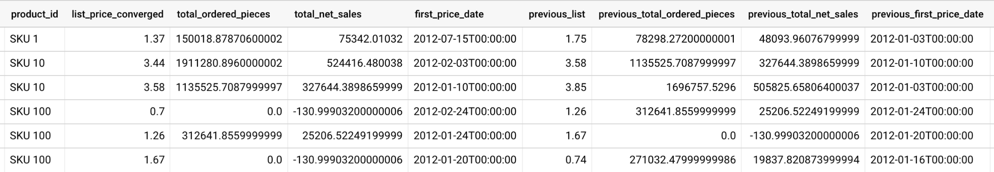
- প্রথমে, আপনাকে একটি অস্থায়ী টেবিল তৈরি করতে হবে যেখানে প্রতিটি পণ্যের মূল্য পরিবর্তনের জন্য একটি করে লাইন থাকবে। এই লাইনে সেই নির্দিষ্ট পণ্যের মূল্য নির্ধারণ সংক্রান্ত তথ্য থাকবে, যেমন প্রতিটি মূল্যে কতগুলো আইটেম অর্ডার করা হয়েছিল এবং সেই মূল্যের সাথে সম্পর্কিত মোট নিট বিক্রয় কত ছিল।
create temp table price_changes as (
select
       product_id,
       list_price_converged,
       total_ordered_pieces,
       total_net_sales,
       first_price_date,
       lag(list_price_converged) over(partition by product_id order by first_price_date asc) as previous_list,
       lag(total_ordered_pieces) over(partition by product_id order by first_price_date asc) as previous_total_ordered_pieces,
       lag(total_net_sales) over(partition by product_id order by first_price_date asc) as previous_total_net_sales,
       lag(first_price_date) over(partition by product_id order by first_price_date asc) as previous_first_price_date
       from (
           select
               product_id,list_price_converged,sum(invoiced_quantity_in_pieces) as total_ordered_pieces, sum(net_sales) as total_net_sales, min(fiscal_date) as first_price_date
           from `{{my_project}}.{{my_dataset}}.CDM_Pricing` AS cdm_pricing
           group by 1,2
           order by 1, 2 asc
       )
);
select * from price_changes where previous_list is not null order by product_id, first_price_date desc
- এরপরে, অস্থায়ী টেবিলটি তৈরি করে, আপনি SKU-গুলো জুড়ে গড় মূল্য পরিবর্তন গণনা করতে পারেন:
select avg((previous_list-list_price_converged)/nullif(previous_list,0))*100 as average_price_change from price_changes;
- অবশেষে, প্রতিটি মূল্য পরিবর্তন এবং অর্ডার করা মোট পণ্যের পরিমাণের মধ্যে সম্পর্কটি খতিয়ে দেখে আপনি বিশ্লেষণ করতে পারেন যে মূল্য পরিবর্তনের পরে কী ঘটে:
select
(total_ordered_pieces-previous_total_ordered_pieces)/nullif(previous_total_ordered_pieces,0)
যেমন
price_changes_percent_ordered_change,
(list_price_converged-previous_list)/nullif(previous_list,0)
যেমন
price_changes_percent_price_change
from price_changes
১২. একটি সময় সিরিজ পূর্বাভাস মডেল তৈরি করুন।
এরপর, BigQuery-এর অন্তর্নির্মিত মেশিন লার্নিং সক্ষমতা ব্যবহার করে, আপনি প্রতিটি পণ্যের বিক্রিত পরিমাণ ভবিষ্যদ্বাণী করার জন্য একটি ARIMA টাইম সিরিজ পূর্বাভাস মডেল তৈরি করতে পারেন।
- প্রথমে আপনাকে একটি ARIMA_PLUS মডেল তৈরি করতে হবে ।
create or replace `{{my_project}}.{{my_dataset}}.bqml_arima`
options
 (model_type = 'ARIMA_PLUS',
  time_series_timestamp_col = 'fiscal_date',
  time_series_data_col = 'total_quantity',
  time_series_id_col = 'product_id',
  auto_arima = TRUE,
  data_frequency = 'AUTO_FREQUENCY',
  decompose_time_series = TRUE
 ) as
select
 fiscal_date,
 product_id,
 sum(invoiced_quantity_in_pieces) as total_quantity
from
 `{{my_project}}.{{my_dataset}}.CDM_Pricing`
group by 1,2;
- এরপরে, আপনি প্রতিটি পণ্যের ভবিষ্যৎ বিক্রয়ের পূর্বাভাস দিতে ML.FORECAST ফাংশনটি ব্যবহার করবেন:
select
*
from
ML.FORECAST(model testing.bqml_arima,
            struct(30 as horizon, 0.8 as confidence_level));
- এই পূর্বাভাসগুলো হাতে থাকলে, দাম বাড়ালে কী হতে পারে তা আপনি বোঝার চেষ্টা করতে পারেন। উদাহরণস্বরূপ, যদি আপনি প্রতিটি পণ্যের দাম ১৫% বাড়ান, তাহলে এই ধরনের একটি কোয়েরি ব্যবহার করে পরবর্তী মাসের আনুমানিক মোট রাজস্ব গণনা করতে পারবেন:
select
sum(forecast_value * list_price) as total_revenue
from ml.forecast(mode testing.bqml_arima,
            struct(30 as horizon, 0.8 as confidence_level)) forecasts
left join (select product_id,
                array_agg(list_price_converged
                       order by fiscal_date desc limit 1)[offset(0)] as list_price
                from `leigha-bq-dev.retail.cdm_pricing` group by 1)  recent_prices
using (product_id);
১৩. একটি প্রতিবেদন তৈরি করুন
এখন যেহেতু আপনার ডি-নরম্যালাইজড প্রাইসিং ডেটা BigQuery-তে কেন্দ্রীভূত করা হয়েছে এবং আপনি এই ডেটার উপর কীভাবে অর্থপূর্ণ কোয়েরি চালাতে হয় তা বুঝে গেছেন, তাই ব্যবসায়িক ব্যবহারকারীদের এই তথ্য অন্বেষণ করতে এবং এর উপর ভিত্তি করে পদক্ষেপ নিতে সক্ষম করার জন্য একটি রিপোর্ট তৈরি করার সময় এসেছে।
আপনার যদি আগে থেকেই একটি Looker ইনস্ট্যান্স থাকে, তাহলে এই প্যাটার্নের প্রাইসিং ডেটা বিশ্লেষণ শুরু করার জন্য আপনি এই GitHub রিপোজিটরিতে থাকা LookML ব্যবহার করতে পারেন। শুধু একটি নতুন Looker প্রজেক্ট তৈরি করুন , LookML- টি যোগ করুন, এবং আপনার BigQuery কনফিগারেশনের সাথে মেলানোর জন্য প্রতিটি ভিউ ফাইলের কানেকশন ও টেবিলের নাম পরিবর্তন করুন।
এই মডেলে, মূল্যের পরিবর্তন পরীক্ষা করার জন্য আপনি সেই ডিরাইভড টেবিলটি ( এই ভিউ ফাইলে ) পাবেন, যা আমরা আগে দেখিয়েছিলাম :
view: price_changes {
    derived_table: {
      sql: select
        product_id,
        list_price_converged,
        total_ordered_pieces,
        total_net_sales,
        first_price_date,
        lag(list_price_converged) over(partition by product_id order by first_price_date asc) as previous_list,
        lag(total_ordered_pieces) over(partition by product_id order by first_price_date asc) as previous_total_ordered_pieces,
        lag(total_net_sales) over(partition by product_id order by first_price_date asc) as previous_total_net_sales,
        lag(first_price_date) over(partition by product_id order by first_price_date asc) as previous_first_price_date
        from (
      select
         product_id,list_price_converged,sum(invoiced_quantity_in_pieces) as total_ordered_pieces, sum(net_sales) as total_net_sales, min(fiscal_date) as first_price_date
      from ${cdm_pricing.SQL_TABLE_NAME}  AS cdm_pricing
      group by 1,2
      order by 1, 2 asc
      )
       ;;
    }
...
}
আমরা আগে যে BigQuery ML ARIMA মডেলটি দেখিয়েছিলাম , তার পাশাপাশি ভবিষ্যৎ বিক্রয়ের পূর্বাভাস দেওয়ার জন্য ( এই ভিউ ফাইলে )
view: arima_model {
  derived_table: {
    persist_for: "24 hours"
    sql_create:
      create or replace model ${sql_table_name}
            options
              (model_type = 'arima_plus',
               time_series_timestamp_col = 'fiscal_date',
               time_series_data_col = 'total_quantity',
               time_series_id_col = 'product_id',
               auto_arima = true,
               data_frequency = 'auto_frequency',
               decompose_time_series = true
              ) as
            select
              fiscal_date,
              product_id,
              sum(invoiced_quantity_in_pieces) as total_quantity
            from
              ${cdm_pricing.sql_table_name}
            group by 1,2 ;;
          }
   }
...
}
LookML-এ একটি নমুনা ড্যাশবোর্ডও রয়েছে। আপনি এখানে ড্যাশবোর্ডটির একটি ডেমো সংস্করণ দেখতে পারেন। ড্যাশবোর্ডের প্রথম অংশটি ব্যবহারকারীদের বিক্রয়, খরচ, মূল্য নির্ধারণ এবং মার্জিনের পরিবর্তন সম্পর্কে উচ্চ-স্তরের তথ্য প্রদান করে। একজন ব্যবসায়িক ব্যবহারকারী হিসেবে, আপনি একটি অ্যালার্ট তৈরি করতে চাইতে পারেন এটা জানার জন্য যে বিক্রয় X%-এর নিচে নেমে গেছে কিনা, কারণ এর অর্থ হতে পারে যে আপনার দাম কমানো উচিত।

পরবর্তী বিভাগটি, যা নিচে দেখানো হয়েছে, ব্যবহারকারীদের মূল্য পরিবর্তনের প্রবণতাগুলো গভীরভাবে খতিয়ে দেখার সুযোগ দেয়। এখানে, আপনি নির্দিষ্ট পণ্যের সঠিক তালিকা মূল্য এবং কী দামে পরিবর্তন করা হয়েছে তা দেখতে পারবেন — যা আরও গবেষণার জন্য নির্দিষ্ট পণ্য চিহ্নিত করতে সহায়ক হতে পারে।

অবশেষে, রিপোর্টের একেবারে নিচে আপনি আমাদের BigQueryML মডেলের ফলাফল দেখতে পাবেন। Looker ড্যাশবোর্ডের উপরের ফিল্টারগুলো ব্যবহার করে, আপনি উপরে বর্ণিত বিভিন্ন পরিস্থিতির অনুরূপ পরিস্থিতি অনুকরণ করার জন্য সহজেই প্যারামিটার প্রবেশ করাতে পারেন। উদাহরণস্বরূপ, নিচে দেখানো অনুযায়ী, যদি অর্ডারের পরিমাণ পূর্বাভাসিত মানের ৭৫%-এ নেমে আসে এবং সমস্ত পণ্যের দাম ২৫% বাড়ানো হয়, তাহলে কী ঘটবে তা দেখতে পারেন।
এটি LookML-এর প্যারামিটার দ্বারা চালিত হয়, যা সরাসরি এখানকার পরিমাপ গণনার মধ্যে অন্তর্ভুক্ত করা হয়। এই ধরনের রিপোর্টিংয়ের মাধ্যমে, আপনি সমস্ত পণ্যের জন্য সর্বোত্তম মূল্য নির্ধারণ করতে পারেন অথবা নির্দিষ্ট পণ্যের গভীরে গিয়ে নির্ধারণ করতে পারেন যে কোথায় আপনার দাম বাড়ানো বা কমানো উচিত এবং এর ফলে মোট ও নীট আয়ের উপর কী প্রভাব পড়বে।
১৪. আপনার মূল্য নির্ধারণ পদ্ধতির সাথে খাপ খাইয়ে নিন
যদিও এই টিউটোরিয়ালটি নমুনা ডেটা সোর্স রূপান্তর করে, আপনার বিভিন্ন প্ল্যাটফর্মে থাকা প্রাইসিং অ্যাসেটগুলোর ক্ষেত্রেও আপনি প্রায় একই ধরনের ডেটা সংক্রান্ত চ্যালেঞ্জের সম্মুখীন হবেন। প্রাইসিং অ্যাসেটগুলোর সারসংক্ষেপ এবং বিস্তারিত ফলাফলের জন্য বিভিন্ন এক্সপোর্ট ফরম্যাট (প্রায়শই xls, sheets, csv, txt, রিলেশনাল ডেটাবেস, বিজনেস অ্যাপ্লিকেশন) থাকে, যার প্রত্যেকটিই ডেটাপ্রেপের সাথে সংযুক্ত করা যায়। আমরা আপনাকে পরামর্শ দিচ্ছি যে, উপরে দেওয়া উদাহরণগুলোর মতোই আপনার রূপান্তরের প্রয়োজনীয়তাগুলো বর্ণনা করে কাজ শুরু করুন। আপনার স্পেসিফিকেশনগুলো স্পষ্ট হয়ে গেলে এবং প্রয়োজনীয় রূপান্তরের ধরনগুলো শনাক্ত করার পর, আপনি ডেটাপ্রেপ ব্যবহার করে সেগুলো ডিজাইন করতে পারবেন।
- যে ডেটাপ্রেপ ফ্লো-টি আপনি কাস্টমাইজ করবেন, সেটির একটি কপি তৈরি করুন (ফ্লো-টির ডানদিকে থাকা ‘more’ বাটনে ক্লিক করে ‘Duplicate’ অপশনটি বেছে নিন), অথবা একেবারে নতুন একটি ডেটাপ্রেপ ফ্লো ব্যবহার করে শুরু থেকে কাজ করুন।
- আপনার নিজস্ব প্রাইসিং ডেটাসেটের সাথে সংযোগ করুন। ডেটাপ্রেপ এক্সেল, সিএসভি, গুগল শিটস, জেএসওএন-এর মতো ফাইল ফরম্যাটগুলো স্বাভাবিকভাবেই সমর্থন করে। আপনি ডেটাপ্রেপ কানেক্টর ব্যবহার করে অন্যান্য সিস্টেমের সাথেও সংযোগ করতে পারেন।
- আপনার চিহ্নিত করা বিভিন্ন রূপান্তর বিভাগে আপনার ডেটা অ্যাসেটগুলো প্রেরণ করুন। প্রতিটি বিভাগের জন্য একটি করে রেসিপি তৈরি করুন। ডেটা রূপান্তর করতে এবং আপনার নিজস্ব রেসিপি লিখতে এই ডিজাইন প্যাটার্নে প্রদত্ত ফ্লো থেকে অনুপ্রেরণা নিন। যদি আপনি আটকে যান, চিন্তা করবেন না, ডেটাপ্রেপ স্ক্রিনের নীচে বাম দিকের চ্যাট ডায়ালগে সাহায্যের জন্য জিজ্ঞাসা করুন।
- আপনার রেসিপিটি আপনার BigQuery ইনস্ট্যান্সের সাথে সংযুক্ত করুন। BigQuery-তে ম্যানুয়ালি টেবিল তৈরি করার বিষয়ে আপনাকে চিন্তা করতে হবে না, Dataprep স্বয়ংক্রিয়ভাবে আপনার জন্য এটি করে দেবে। আমরা পরামর্শ দিই যে, যখন আপনি আপনার ফ্লো-তে আউটপুট যোগ করবেন, তখন একটি ম্যানুয়াল ডেস্টিনেশন নির্বাচন করুন এবং প্রতিটি রানে টেবিলটি ড্রপ করুন। প্রত্যাশিত ফলাফল না পাওয়া পর্যন্ত প্রতিটি রেসিপি আলাদাভাবে পরীক্ষা করুন। আপনার পরীক্ষা শেষ হয়ে গেলে, পূর্ববর্তী ডেটা মুছে যাওয়া এড়াতে প্রতিটি রানে আউটপুটটি টেবিলে অ্যাপেন্ড করার জন্য রূপান্তর করুন।
- আপনি চাইলে ফ্লো-টিকে একটি নির্দিষ্ট সময়সূচী অনুযায়ী চালানোর জন্য যুক্ত করতে পারেন। আপনার প্রসেসটি যদি অবিচ্ছিন্নভাবে চলার প্রয়োজন হয়, তবে এটি একটি কার্যকরী বিষয়। আপনার প্রয়োজনীয় সতেজতার উপর ভিত্তি করে, আপনি প্রতিদিন বা প্রতি ঘণ্টায় রেসপন্স লোড করার জন্য একটি সময়সূচী নির্ধারণ করতে পারেন। আপনি যদি ফ্লো-টি একটি নির্দিষ্ট সময়সূচী অনুযায়ী চালানোর সিদ্ধান্ত নেন, তবে প্রতিটি রেসিপির জন্য ফ্লো-তে একটি 'Schedule Destination Output' যোগ করতে হবে।
BigQuery মেশিন লার্নিং মডেলটি পরিবর্তন করুন
এই টিউটোরিয়ালে একটি নমুনা ARIMA মডেল দেওয়া হয়েছে। তবে, মডেলটি তৈরি করার সময় আপনি আরও কিছু প্যারামিটার নিয়ন্ত্রণ করতে পারেন, যাতে এটি আপনার ডেটার সাথে সবচেয়ে ভালোভাবে খাপ খায়। আপনি এখানে আমাদের ডকুমেন্টেশনের মধ্যে থাকা উদাহরণটিতে আরও বিস্তারিত দেখতে পারেন। এছাড়াও, আপনি আপনার মডেল সম্পর্কে আরও বিস্তারিত জানতে এবং অপটিমাইজেশনের সিদ্ধান্ত নিতে BigQuery-এর ML.ARIMA_EVALUATE , ML.ARIMA_COEFFICIENTS , এবং ML.EXPLAIN_FORECAST ফাংশনগুলোও ব্যবহার করতে পারেন।
লুকার রিপোর্ট সম্পাদনা করুন
উপরে বর্ণিত পদ্ধতি অনুযায়ী আপনার নিজের প্রোজেক্টে LookML ইম্পোর্ট করার পর, আপনি সরাসরি সম্পাদনা করে অতিরিক্ত ফিল্ড যোগ করতে, ক্যালকুলেশন বা ব্যবহারকারীর দেওয়া প্যারামিটার পরিবর্তন করতে এবং আপনার ব্যবসার প্রয়োজন অনুসারে ড্যাশবোর্ডের ভিজ্যুয়ালাইজেশনগুলো বদলাতে পারবেন। LookML-এ ডেভেলপ করার বিস্তারিত তথ্য আপনি এখানে এবং Looker-এ ডেটা ভিজ্যুয়ালাইজ করার বিস্তারিত তথ্য এখানে পাবেন।
১৫. অভিনন্দন
আপনার খুচরা পণ্যের মূল্য নির্ধারণ অপ্টিমাইজ করার জন্য প্রয়োজনীয় মূল পদক্ষেপগুলো এখন আপনি জানেন!
এরপর কী?
অন্যান্য স্মার্ট অ্যানালিটিক্স রেফারেন্স প্যাটার্নগুলি অন্বেষণ করুন
আরও পড়ুন
- ব্লগটি এখানে পড়ুন
- ডেটাপ্রেপ সম্পর্কে এখানে আরও জানুন।
- BigQuery মেশিন লার্নিং সম্পর্কে এখানে আরও জানুন।
- লুকার সম্পর্কে এখানে আরও জানুন