
1. Introduction
Last Updated: 2022-07-14
Observability of the application
Observability and Continuous Profiler
Observability is the term used to describe an attribute of a system. A system with observability allows teams to actively debug their system. In that context, three pillars of observability; logs, metrics, and traces are the fundamental instrumentation for the system to acquire observability.
Also in addition to the three pillars of observability, continuous profiling is another key component for observability and it is expandings the user base in the industry. Cloud Profiler is one of the originators and provides an easy interface to drill down the performance metrics in the application call stacks.
This codelab is part 2 of the series and covers instrumenting a continuous profiler agent. Part 1 covers distributed tracing with OpenTelemetry and Cloud Trace, and you will learn more about identifying the bottleneck of the microservices better with part 1.
What you'll build
In this codelab, you're going to instrument continuous profiler agent in the server service of "Shakespeare application" (a.k.a. Shakesapp) that runs on a Google Kubernetes Engine cluster. The architecture of Shakesapp is as described below:
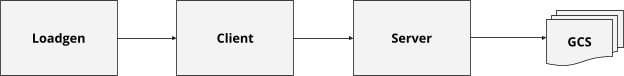
- Loadgen sends a query string to the client in HTTP
- Clients pass through the query from the loadgen to the server in gRPC
- Server accepts the query from the client, fetches all Shakespare works in text format from Google Cloud Storage, searches the lines that contain the query and return the number of the line that matched to the client
In part 1, you found that the bottleneck exists somewhere in the server service, but you could not identify the exact cause.
What you'll learn
- How to embed profiler agent
- How to investigate the bottle neck on Cloud Profiler
This codelab explains how to instrument a continuous profiler agent in your application.
What you'll need
- A basic knowledge of Go
- A basic knowledge of Kubernetes
2. Setup and Requirements
Self-paced environment setup
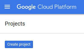
If you don't already have a Google Account (Gmail or Google Apps), you must create one. Sign-in to Google Cloud Platform console ( console.cloud.google.com) and create a new project.
If you already have a project, click on the project selection pull down menu in the upper left of the console:
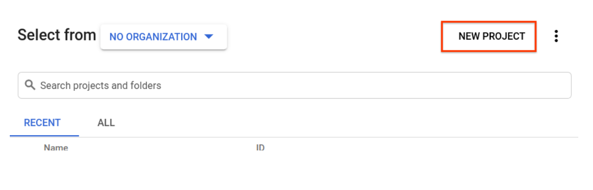
and click the ‘NEW PROJECT' button in the resulting dialog to create a new project:
If you don't already have a project, you should see a dialog like this to create your first one:
The subsequent project creation dialog allows you to enter the details of your new project:
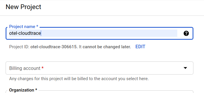
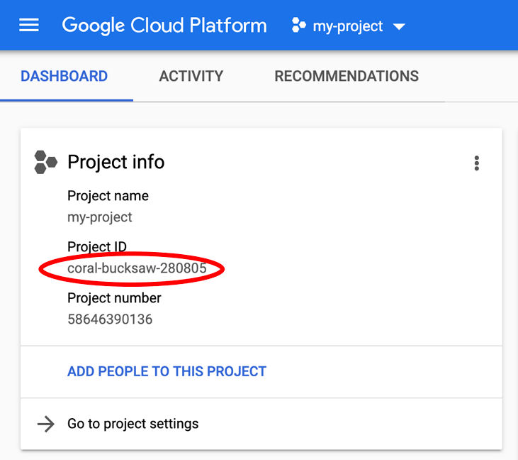
Remember the project ID, which is a unique name across all Google Cloud projects (the name above has already been taken and will not work for you, sorry!). It will be referred to later in this codelab as PROJECT_ID.
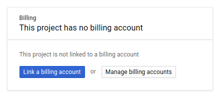
Next, if you haven't already done so, you'll need to enable billing in the Developers Console in order to use Google Cloud resources and enable the Cloud Trace API.
Running through this codelab shouldn't cost you more than a few dollars, but it could be more if you decide to use more resources or if you leave them running (see "cleanup" section at the end of this document). Pricings of Google Cloud Trace, Google Kubernetes Engine and Google Artifact Registry are noted on the official documentation.
- Pricing for Google Cloud's operations suite | Operations Suite
- Pricing | Kubernetes Engine Documentation
- Artifact Registry Pricing | Artifact Registry documentation
New users of Google Cloud Platform are eligible for a $300 free trial, which should make this codelab entirely free of charge.
Google Cloud Shell Setup
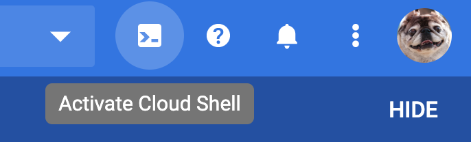
While Google Cloud and Google Cloud Trace can be operated remotely from your laptop, in this codelab we will be using Google Cloud Shell, a command line environment running in the Cloud.
This Debian-based virtual machine is loaded with all the development tools you'll need. It offers a persistent 5GB home directory and runs in Google Cloud, greatly enhancing network performance and authentication. This means that all you will need for this codelab is a browser (yes, it works on a Chromebook).
To activate Cloud Shell from the Cloud Console, simply click Activate Cloud Shell  (it should only take a few moments to provision and connect to the environment).
Once connected to Cloud Shell, you should see that you are already authenticated and that the project is already set to your PROJECT_ID.
gcloud auth list
Command output
Credentialed accounts:
 - <myaccount>@<mydomain>.com (active)
gcloud config list project
Command output
[core]
project = <PROJECT_ID>
If, for some reason, the project is not set, simply issue the following command:
gcloud config set project <PROJECT_ID>
Looking for your PROJECT_ID? Check out what ID you used in the setup steps or look it up in the Cloud Console dashboard:
Cloud Shell also sets some environment variables by default, which may be useful as you run future commands.
echo $GOOGLE_CLOUD_PROJECT
Command output
<PROJECT_ID>
Finally, set the default zone and project configuration.
gcloud config set compute/zone us-central1-f
You can choose a variety of different zones. For more information, see Regions & Zones.
Go language setup
In this codelab, we use Go for all source code. Run the following command on Cloud Shell and confirm if the Go's version is 1.17+
go version
Command output
go version go1.18.3 linux/amd64
Setup a Google Kubernetes Cluster
In this codelab, you will run a cluster of microservices on Google Kubernetes Engine (GKE). The process of this codelab is as the following:
- Download the baseline project into Cloud Shell
- Build microservices into containers
- Upload containers onto Google Artifact Registry (GAR)
- Deploy containers onto GKE
- Modify the source code of services for trace instrumentation
- Go to step2
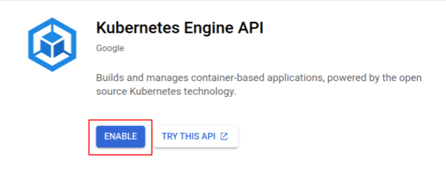
Enable Kubernetes Engine
First, we set up a Kubernetes cluster where Shakesapp runs on GKE, so we need to enable GKE. Navigate to the menu "Kubernetes Engine" and press the ENABLE button.
Now you are ready to create a Kubernetes cluster.
Create Kubernetes cluster
On Cloud Shell, run the following command to create a Kubernetes cluster. Please confirm the zone value is under the region that you will use for Artifact Registry repository creation. Change the zone value us-central1-f if your repository region is not covering the zone.
gcloud container clusters create otel-trace-codelab2 \
--zone us-central1-f \
--release-channel rapid \
--preemptible \
--enable-autoscaling \
--max-nodes 8 \
--no-enable-ip-alias \
--scopes cloud-platform
Command output
Note: Your Pod address range (`--cluster-ipv4-cidr`) can accommodate at most 1008 node(s).
Creating cluster otel-trace-codelab2 in us-central1-f... Cluster is being health-checked (master is healthy)...done.
Created [https://container.googleapis.com/v1/projects/development-215403/zones/us-central1-f/clusters/otel-trace-codelab2].
To inspect the contents of your cluster, go to: https://console.cloud.google.com/kubernetes/workload_/gcloud/us-central1-f/otel-trace-codelab2?project=development-215403
kubeconfig entry generated for otel-trace-codelab2.
NAME: otel-trace-codelab2
LOCATION: us-central1-f
MASTER_VERSION: 1.23.6-gke.1501
MASTER_IP: 104.154.76.89
MACHINE_TYPE: e2-medium
NODE_VERSION: 1.23.6-gke.1501
NUM_NODES: 3
STATUS: RUNNING
Artifact Registry and skaffold setup
Now we have a Kubernetes cluster ready for deployment. Next we prepare for a container registry for push and deploy containers. For these steps, we need to set up an Artifact Registry (GAR) and skaffold to use it.
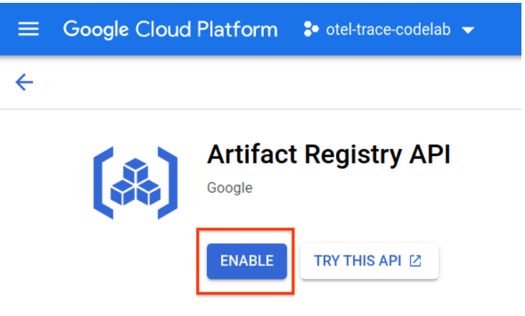
Artifact Registry setup
Navigate to the menu of "Artifact Registry" and press the ENABLE button.
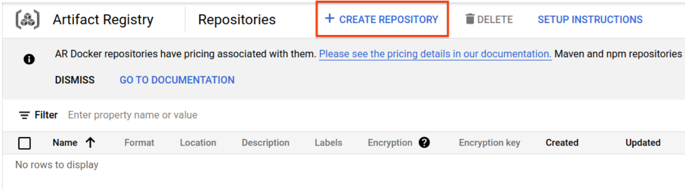
After some moments, you will see the repository browser of GAR. Click the "CREATE REPOSITORY" button and enter the name of the repository.
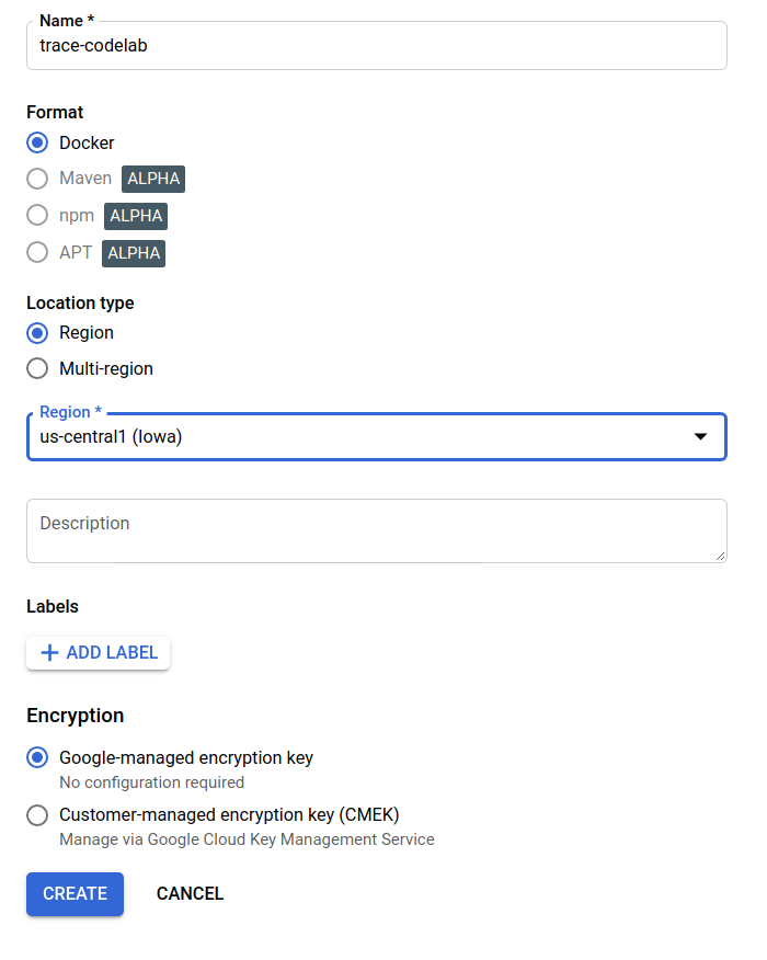
In this codelab, I name the new repository trace-codelab. The format of the artifact is "Docker" and the location type is "Region". Choose the region close to the one you set for Google Compute Engine default zone. For example, this example chose "us-central1-f" above, so here we choose "us-central1 (Iowa)". Then click the "CREATE" button.
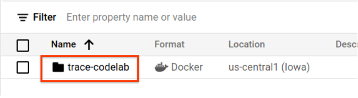
Now you see "trace-codelab" on the repository browser.
We will come back here later to check the registry path.
Skaffold setup
Skaffold is a handy tool when you work on building microservices that run on Kubernetes. It handles the workflow of building, pushing and deploying containers of applications with a small set of commands. Skaffold by default uses Docker Registry as container registry, so you need to configure skaffold to recognize GAR on pushing containers to.
Open Cloud Shell again and confirm if skaffold is installed. (Cloud Shell installs skaffold into the environment by default.) Run the following command and see the skaffold version.
skaffold version
Command output
v1.38.0
Now, you can register the default repository for skaffold to use. In order to obtain the registry path, navigate yourself to the Artifact Registry dashboard and click the name of the repository you just set up in the previous step.
Then you will see breadcrumbs trails on the top of the page. Click  icon to copy the registry path to the clipboard.
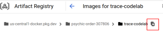
On clicking the copy button, you see the dialog at the bottom of the browser with the message like:
"us-central1-docker.pkg.dev/psychic-order-307806/trace-codelab" has been copied
Go back to the cloud shell. Run skaffold config set default-repo command with the value you just copied from the dashboard.
skaffold config set default-repo us-central1-docker.pkg.dev/psychic-order-307806/trace-codelab
Command output
set value default-repo to us-central1-docker.pkg.dev/psychic-order-307806/trace-codelab for context gke_stackdriver-sandbox-3438851889_us-central1-b_stackdriver-sandbox
Also, you need to configure the registry to Docker configuration. Run the following command:
gcloud auth configure-docker us-central1-docker.pkg.dev --quiet
Command output
{
  "credHelpers": {
    "gcr.io": "gcloud",
    "us.gcr.io": "gcloud",
    "eu.gcr.io": "gcloud",
    "asia.gcr.io": "gcloud",
    "staging-k8s.gcr.io": "gcloud",
    "marketplace.gcr.io": "gcloud",
    "us-central1-docker.pkg.dev": "gcloud"
  }
}
Adding credentials for: us-central1-docker.pkg.dev
Now you are good to go for the next step to set up a Kubernetes container on GKE.
Summary
In this step, you set up your codelab environment:
- Set up Cloud Shell
- Created a Artifact Registry repository for the container registry
- Set up skaffold to use the container registry
- Created a Kubernetes cluster where the codelab microservices run
Next up
In the next step, you will instrument continuous profiler agent in the server service.
3. Build, push and deploy the microservices
Download the codelab material
In the previous step, we have set up all prerequisites for this codelab. Now you are ready to run whole microservices on top of them. The codelab material is hosted on GitHub, so download them to the Cloud Shell environment with the following git command.
cd ~
git clone https://github.com/ymotongpoo/opentelemetry-trace-codelab-go.git
cd opentelemetry-trace-codelab-go
The directory structure of the project is as the followings:
.
├── README.md
├── step0
│   ├── manifests
│   ├── proto
│   ├── skaffold.yaml
│   └── src
├── step1
│   ├── manifests
│   ├── proto
│   ├── skaffold.yaml
│   └── src
├── step2
│   ├── manifests
│   ├── proto
│   ├── skaffold.yaml
│   └── src
├── step3
│   ├── manifests
│   ├── proto
│   ├── skaffold.yaml
│   └── src
├── step4
│   ├── manifests
│   ├── proto
│   ├── skaffold.yaml
│   └── src
├── step5
│   ├── manifests
│   ├── proto
│   ├── skaffold.yaml
│   └── src
└── step6
    ├── manifests
    ├── proto
    ├── skaffold.yaml
    └── src
- manifests: Kubernetes manifest files
- proto: proto definition for the communication between client and server
- src: directories for the source code of each services
- skaffold.yaml: Configuration file for skaffold
In this codelab, you will update the source code located under step4 folder. You can also refer to the source code in step[1-6] folders for the changes from the beginning. (Part 1 covers step0 to step4, and Part 2 covers step 5 and 6)
Run skaffold command
Finally you are ready to build, push and deploy whole content onto the Kubernetes cluster you have just created. This sounds like it contains multiple steps but the actual is skaffold does everything for you. Let's try that with the following command:
cd step4
skaffold dev
As soon as running the command, you see the log output of docker build and can confirm that they are successfully pushed to the registry.
Command output
...
---> Running in c39b3ea8692b
 ---> 90932a583ab6
Successfully built 90932a583ab6
Successfully tagged us-central1-docker.pkg.dev/psychic-order-307806/trace-codelab/serverservice:step1
The push refers to repository [us-central1-docker.pkg.dev/psychic-order-307806/trace-codelab/serverservice]
cc8f5a05df4a: Preparing
5bf719419ee2: Preparing
2901929ad341: Preparing
88d9943798ba: Preparing
b0fdf826a39a: Preparing
3c9c1e0b1647: Preparing
f3427ce9393d: Preparing
14a1ca976738: Preparing
f3427ce9393d: Waiting
14a1ca976738: Waiting
3c9c1e0b1647: Waiting
b0fdf826a39a: Layer already exists
88d9943798ba: Layer already exists
f3427ce9393d: Layer already exists
3c9c1e0b1647: Layer already exists
14a1ca976738: Layer already exists
2901929ad341: Pushed
5bf719419ee2: Pushed
cc8f5a05df4a: Pushed
step1: digest: sha256:8acdbe3a453001f120fb22c11c4f6d64c2451347732f4f271d746c2e4d193bbe size: 2001
After the push of all service containers, Kubernetes deployments start automatically.
Command output
sha256:b71fce0a96cea08075dc20758ae561cf78c83ff656b04d211ffa00cedb77edf8 size: 1997
Tags used in deployment:
 - serverservice -> us-central1-docker.pkg.dev/psychic-order-307806/trace-codelab/serverservice:step4@sha256:8acdbe3a453001f120fb22c11c4f6d64c2451347732f4f271d746c2e4d193bbe
 - clientservice -> us-central1-docker.pkg.dev/psychic-order-307806/trace-codelab/clientservice:step4@sha256:b71fce0a96cea08075dc20758ae561cf78c83ff656b04d211ffa00cedb77edf8
 - loadgen -> us-central1-docker.pkg.dev/psychic-order-307806/trace-codelab/loadgen:step4@sha256:eea2e5bc8463ecf886f958a86906cab896e9e2e380a0eb143deaeaca40f7888a
Starting deploy...
 - deployment.apps/clientservice created
 - service/clientservice created
 - deployment.apps/loadgen created
 - deployment.apps/serverservice created
 - service/serverservice created
After the deployment, you'll see the actual application logs emitted to stdout in each containers like this:
Command output
[client] 2022/07/14 06:33:15 {"match_count":3040}
[loadgen] 2022/07/14 06:33:15 query 'love': matched 3040
[client] 2022/07/14 06:33:15 {"match_count":3040}
[loadgen] 2022/07/14 06:33:15 query 'love': matched 3040
[client] 2022/07/14 06:33:16 {"match_count":3040}
[loadgen] 2022/07/14 06:33:16 query 'love': matched 3040
[client] 2022/07/14 06:33:19 {"match_count":463}
[loadgen] 2022/07/14 06:33:19 query 'tear': matched 463
[loadgen] 2022/07/14 06:33:20 query 'world': matched 728
[client] 2022/07/14 06:33:20 {"match_count":728}
[client] 2022/07/14 06:33:22 {"match_count":463}
[loadgen] 2022/07/14 06:33:22 query 'tear': matched 463
Note that at this point, you want to see any messages from the server. OK, finally you are ready to start instrumenting your application with OpenTelemetry for distributed tracing of the services.
Before starting instrumenting the service, please shut down your cluster with Ctrl-C.
Command output
...
[client] 2022/07/14 06:34:57 {"match_count":1}
[loadgen] 2022/07/14 06:34:57 query 'what's past is prologue': matched 1
^CCleaning up...
 - W0714 06:34:58.464305   28078 gcp.go:120] WARNING: the gcp auth plugin is deprecated in v1.22+, unavailable in v1.25+; use gcloud instead.
 - To learn more, consult https://cloud.google.com/blog/products/containers-kubernetes/kubectl-auth-changes-in-gke
 - deployment.apps "clientservice" deleted
 - service "clientservice" deleted
 - deployment.apps "loadgen" deleted
 - deployment.apps "serverservice" deleted
 - service "serverservice" deleted
Summary
In this step, you have prepared the codelab material in your environment and confirmed skaffold runs as expected.
Next up
In the next step, you will modify the source code of loadgen service to instrument the trace information.
4. Instrumentation of Cloud Profiler agent
Concept of continuous profiling
Before explaining the concept of continuous profiling, we need to understand that of profiling first. Profiling is the one of the ways to analyze the application dynamically (dynamic program analysis) and is usually performed during the application development in the process of load testing and so on. That is a single shot activity to measure the system metrics, such as CPU and memory usages, during the specific period. After collecting the profile data, developers analyze them off the code.
Continuous profiling is the extended approach of normal profiling: It runs short window profiles against the long running application periodically and collects a bunch of profile data. Then it automatically generates the statistical analysis based on a certain attribute of the application, such as version number, deployment zone, measurement time, and so on. You will find further details of the concept in our documentation.
Because the target is a running application, there's a way to collect profile data periodically and send them to some backend that post-processes the statistical data. That is the Cloud Profiler agent and you are going to embed it to the server service soon.
Embed Cloud Profiler agent
Open Cloud Shell Editor by pressing the button  at the top right of the Cloud Shell. Open
 step4/src/server/main.go from the explorer in the left pane and find the main function.
step4/src/server/main.go
func main() {
        ...
        // step2. setup OpenTelemetry
        tp, err := initTracer()
        if err != nil {
                log.Fatalf("failed to initialize TracerProvider: %v", err)
        }
        defer func() {
                if err := tp.Shutdown(context.Background()); err != nil {
                        log.Fatalf("error shutting down TracerProvider: %v", err)
                }
        }()
        // step2. end setup

        svc := NewServerService()
        // step2: add interceptor
        interceptorOpt := otelgrpc.WithTracerProvider(otel.GetTracerProvider())
        srv := grpc.NewServer(
                grpc.UnaryInterceptor(otelgrpc.UnaryServerInterceptor(interceptorOpt)),
                grpc.StreamInterceptor(otelgrpc.StreamServerInterceptor(interceptorOpt)),
        )
        // step2: end adding interceptor
        shakesapp.RegisterShakespeareServiceServer(srv, svc)
        healthpb.RegisterHealthServer(srv, svc)
        if err := srv.Serve(lis); err != nil {
                log.Fatalf("error serving server: %v", err)
        }
}
In the main function, you see some setup code for OpenTelemetry and gRPC, which has been done in the codelab part 1. Now you will add instrumentation for Cloud Profiler agent here. Like what we did for initTracer() you can write a function called initProfiler() for readability.
step4/src/server/main.go
import (
        ...
        "cloud.google.com/go/profiler" // step5. add profiler package
        "cloud.google.com/go/storage"
        ...
)

// step5: add Profiler initializer
func initProfiler() {
        cfg := profiler.Config{
                Service:              "server",
                ServiceVersion:       "1.0.0",
                NoHeapProfiling:      true,
                NoAllocProfiling:     true,
                NoGoroutineProfiling: true,
                NoCPUProfiling:       false,
        }
        if err := profiler.Start(cfg); err != nil {
                log.Fatalf("failed to launch profiler agent: %v", err)
        }
}
Let's take a close look at the options specified in profiler.Config{} object.
- Service: The service name that you can select and switch on profiler dashboard
- ServiceVersion: The service version name. You can compare profile data sets based on this value.
- NoHeapProfiling: disable memory consumption profiling
- NoAllocProfiling: disable memory allocation profiling
- NoGoroutineProfiling: disable goroutine profiling
- NoCPUProfiling: disable CPU profiling
In this codelab, we only enable CPU profiling.
Now what you need to do is just call this function in the main function. Make sure to import the Cloud Profiler package in the import block.
step4/src/server/main.go
func main() {
        ...
        defer func() {
                if err := tp.Shutdown(context.Background()); err != nil {
                        log.Fatalf("error shutting down TracerProvider: %v", err)
                }
        }()
        // step2. end setup

        // step5. start profiler
        go initProfiler()
        // step5. end

        svc := NewServerService()
        // step2: add interceptor
        ...
}
Note that you are calling the initProfiler() function with the go keyword. Because profiler.Start() blocks so you need to run it in another goroutine. Now it's ready to build. Make sure to run go mod tidy in advance of deployment.
go mod tidy
Now deploy your cluster with your new server service.
skaffold dev
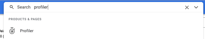
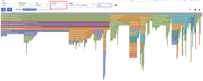
It usually takes a couple of minutes to see the flame graph on Cloud Profiler. Type in "profiler" in the search box at the top and click Profiler's icon.
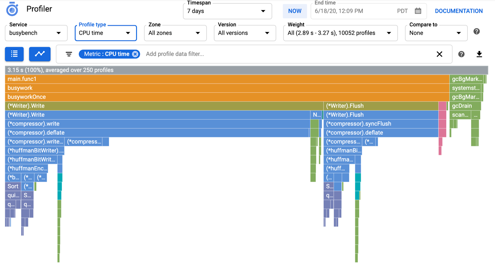
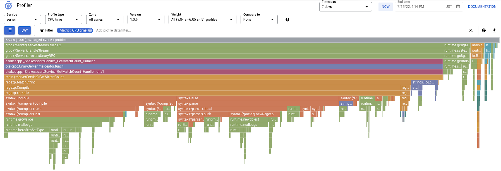
Then you will see the following flame graph.
Summary
In this step, you embedded Cloud Profiler agent to the server service and confirmed that it generates flame graph.
Next up
In the next step, you will investigate the cause of the bottleneck in the application with the flame graph.
5. Analyze Cloud Profiler flame graph
What is Flame Graph?
Flame Graph is one of the ways to visualize the profile data. For detailed explanation, please refer to our document, but the short summary is:
- Each bar expresses the method/function call in the application
- Vertical direction is the call stack; call stack grows from top to bottom
- Horizontal direction is the resource usage; the longer, the worse.
Given that, let's look at the obtained flame graph.
Analyzing Flame Graph
In the previous section, you learned that each bar in the flame graph expresses the function/method call, and the length of it means the resource usage in the function/method. Cloud Profiler's flame graph sorts the bar in the descending order or the length from left to right, you can start looking at the top left of the graph first.
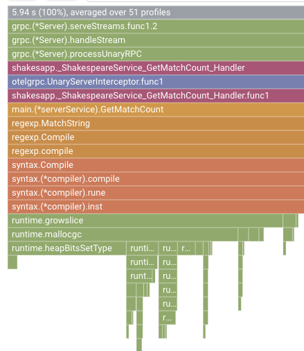
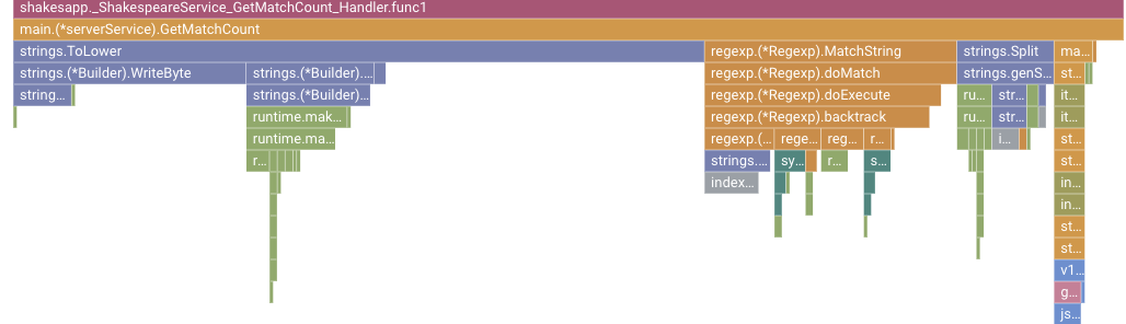
In our case, it is explicit that grpc.(*Server).serveStreams.func1.2 is consuming the most of CPU time, and by looking through the call stack from the top to the bottom, that is spent most of the time in main.(*serverService).GetMatchCount, which is the gRPC server handler in the server service.
Under GetMatchCount, you see a series of regexp functions: regexp.MatchString and regexp.Compile. They are from the standard package: that is, they should be well tested from many points of view, including performance. But the result here shows that CPU time resource usage is high in the regexp.MatchString and regexp.Compile. Given those facts, the assumption here is that the use of regexp.MatchString has something to do with performance issues. So let's read the source code where the function is used.
step4/src/server/main.go
func (s *serverService) GetMatchCount(ctx context.Context, req *shakesapp.ShakespeareRequest) (*shakesapp.ShakespeareResponse, error) {
        resp := &shakesapp.ShakespeareResponse{}
        texts, err := readFiles(ctx, bucketName, bucketPrefix)
        if err != nil {
                return resp, fmt.Errorf("fails to read files: %s", err)
        }
        for _, text := range texts {
                for _, line := range strings.Split(text, "\n") {
                        line, query := strings.ToLower(line), strings.ToLower(req.Query)
                        isMatch, err := regexp.MatchString(query, line)
                        if err != nil {
                                return resp, err
                        }
                        if isMatch {
                                resp.MatchCount++
                        }
                }
        }
        return resp, nil
}
This is the place where regexp.MatchString is called. By reading the source code, you may notice that the function is called inside the nested for-loop. So the use of this function may be incorrect. Let's look up the GoDoc of regexp.
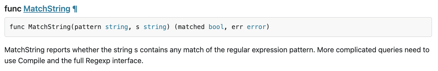
According to the document, regexp.MatchString compiles the regular expression pattern in every call. So the cause of the large resource consumption sounds like this.
Summary
In this step, you made the assumption of the cause of resource consumption by analyzing the flame graph.
Next up
In the next step, you will update the source code of the server service and confirm the change from the version 1.0.0.
6. Update the source code and diff the flame graphs
Update the source code
In the previous step, you made the assumption that the usage of regexp.MatchString has something to do with the large resource consumption. So let's resolve this. Open the code and change that part a bit.
step4/src/server/main.go
func (s *serverService) GetMatchCount(ctx context.Context, req *shakesapp.ShakespeareRequest) (*shakesapp.ShakespeareResponse, error) {
        resp := &shakesapp.ShakespeareResponse{}
        texts, err := readFiles(ctx, bucketName, bucketPrefix)
        if err != nil {
                return resp, fmt.Errorf("fails to read files: %s", err)
        }

        // step6. considered the process carefully and naively tuned up by extracting
        // regexp pattern compile process out of for loop.
        query := strings.ToLower(req.Query)
        re := regexp.MustCompile(query)
        for _, text := range texts {
                for _, line := range strings.Split(text, "\n") {
                        line = strings.ToLower(line)
                        isMatch := re.MatchString(line)
                        // step6. done replacing regexp with strings
                        if isMatch {
                                resp.MatchCount++
                        }
                }
        }
        return resp, nil
}
As you see, now the regexp pattern compilation process is extracted from the regexp.MatchString and is moved out of the nested for loop.
Before deploying this code, make sure to update the version string in initProfiler() function.
step4/src/server/main.go
func initProfiler() {
        cfg := profiler.Config{
                Service:              "server",
                ServiceVersion:       "1.1.0", // step6. update version
                NoHeapProfiling:      true,
                NoAllocProfiling:     true,
                NoGoroutineProfiling: true,
                NoCPUProfiling:       false,
        }
        if err := profiler.Start(cfg); err != nil {
                log.Fatalf("failed to launch profiler agent: %v", err)
        }
}
Now let's see how it works. Deploy the cluster with skaffold command.
skaffold dev
And after a while, reload Cloud Profiler dashboard and see how it is like.
Make sure to change the version to "1.1.0" so that you only see the profiles from version 1.1.0. As you can tell, the length of the bar of GetMatchCount reduced and the usage ratio of CPU time (i.e. the bar got shorter).
Not just by looking at the flame graph of a single version, you can also compare the diffs between two versions.

Change the value of "Compare to" drop down list to "Version" and change the value of "Compared version" to "1.0.0", the original version.
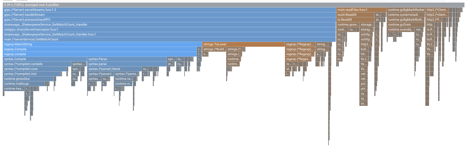
You will see this kind of flame graph. The shape of the graph is the same as 1.1.0 but the coloring is different. In comparison mode, what the color means is:
- Blue: the value (resource consumption) reduced
- Orange: the value (resource consumption) gained
- Gray: neutral
Given the legend, let's take a closer look at the function. By clicking on the bar you want to zoom in, you can see more details inside the stack. Please click main.(*serverService).GetMatchCount bar. Also by hovering over the bar, you will see the details of the comparison.
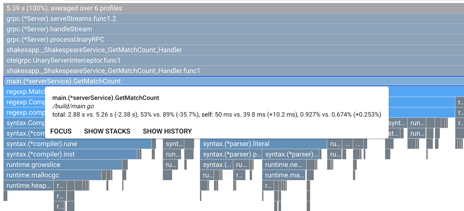
It says the total CPU time is reduced from 5.26s to 2.88s (total is 10s = sampling window). This is a huge improvement!
Now you could improve your application performance from the analysis of profile data.
Summary
In this step, you made an edit in the server service and confirmed the improvement on Cloud Profiler's comparison mode.
Next up
In the next step, you will update the source code of the server service and confirm the change from the version 1.0.0.
7. Extra step: Confirm the improvement in Trace waterfall
Difference between distributed trace and continuous profiling
In part 1 of the codelab, you confirmed that you could figure out the bottleneck service across the microservices for a request path and that you could not figure out the exact cause of the bottleneck in the specific service. In this part 2 codelab, you have learned that continuous profiling enables you to identify the bottleneck inside the single service from call stacks.
In this step, let's review the waterfall graph from the distributed trace (Cloud Trace) and see the difference from the continuous profiling.
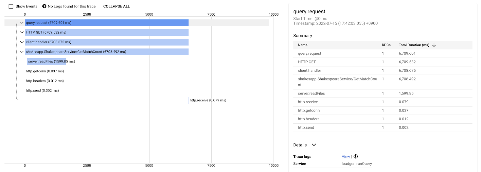
This waterfall graph is the one of the traces with the query "love". It is taking about 6.7s (6700ms) in total.
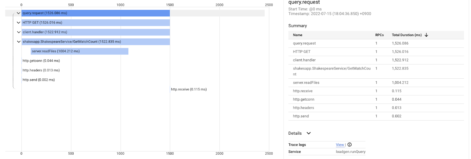
And this is after the improvement for the same query. As you tell, the total latency is now 1.5s (1500ms), which is a huge improvement from the previous implementation.
The important point here is that in the distributed trace waterfall chart, the call stack information is not available unless you instrument spans everywhere around. Also distributed traces just focus on the latency across the services whereas continuous profiling focuses on the computer resources (CPU, memory, OS threads) of a single service.
In another aspect, the distributed trace is the event base, continuous profile is statistical. Each trace has a different latency graph and you need a different format such as distribution to get the trend of latency changes.
Summary
In this step, you checked the difference between distributed trace and continuous profiling.
8. Congratulations
You have successfully created distributed traces with OpenTelemery and confirmed request latencies across the microservice on Google Cloud Trace.
For extended exercises, you can try the following topics by yourself.
- Current implementation sends all spans generated by health check. (
grpc.health.v1.Health/Check) How do you filter out those spans from Cloud Traces? Hint is here. - Correlate event logs with spans and see how it works on Google Cloud Trace and Google Cloud Logging. Hint is here.
- Replace some service with the one in another language and try to instrument it with OpenTelemetry for that language.
Also, if you would like to learn about the profiler after this, please move on to part 2. You can skip the clean up section below in that case.
Clean up
After this codelab, please stop the Kubernetes cluster and make sure to delete the project so that you don't get unexpected charges on Google Kubernetes Engine, Google Cloud Trace, Google Artifact Registry.
First, delete the cluster. If you are running the cluster with skaffold dev, you just need to press Ctrl-C. If you are running the cluster with skaffold run, run the following command:
skaffold delete
Command output
Cleaning up...
 - deployment.apps "clientservice" deleted
 - service "clientservice" deleted
 - deployment.apps "loadgen" deleted
 - deployment.apps "serverservice" deleted
 - service "serverservice" deleted
After deleting the cluster, from the menu pane, select "IAM & Admin" > "Settings", and then click "SHUT DOWN" button.
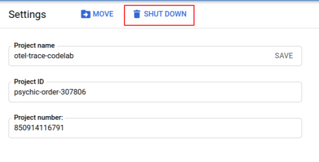
Then enter the Project ID (not Project Name) in the form in the dialog and confirm shutdown.