1. 概要
このラボでは、Google Cloud の新しく発表されたマネージド ML プラットフォームである Vertex AI を使用して、エンドツーエンドの ML ワークフローを構築する方法を学習します。このワークショップでは、生データからデプロイされたモデルまでの流れを学び、Vertex AI を使用して独自の ML プロジェクトを開発し、製品化する準備を整えます。このラボでは、Cloud Shell を使用してカスタム Docker イメージを構築し、Vertex AI でのトレーニング用のカスタム コンテナをデモンストレートします。
ここではモデルのコードに TensorFlow を使用していますが、別のフレームワークに簡単に置き換えることができます。
学習内容
次の方法を学習します。
- Cloud Shell を使用してモデル トレーニング コードをビルドしてコンテナ化する
- カスタムモデルのトレーニング ジョブを Vertex AI に送信する
- トレーニングしたモデルをエンドポイントにデプロイし、そのエンドポイントを使用して予測を行う
このラボを Google Cloud で実行するための総費用は約 $2 です。
2. Vertex AI の概要
このラボでは、Google Cloud で利用できる最新の AI プロダクトを使用します。Vertex AI は Google Cloud 全体の ML サービスを統合してシームレスな開発エクスペリエンスを提供します。以前は、AutoML でトレーニングしたモデルやカスタムモデルにそれぞれ個別のサービスを介してアクセスする必要がありましたが、Vertex AI は、これらの個別のサービスを他の新しいプロダクトとともに 1 つの API にまとめます。既存のプロジェクトを Vertex AI に移行することもできます。ご意見やご質問がありましたら、サポートページからお寄せください。
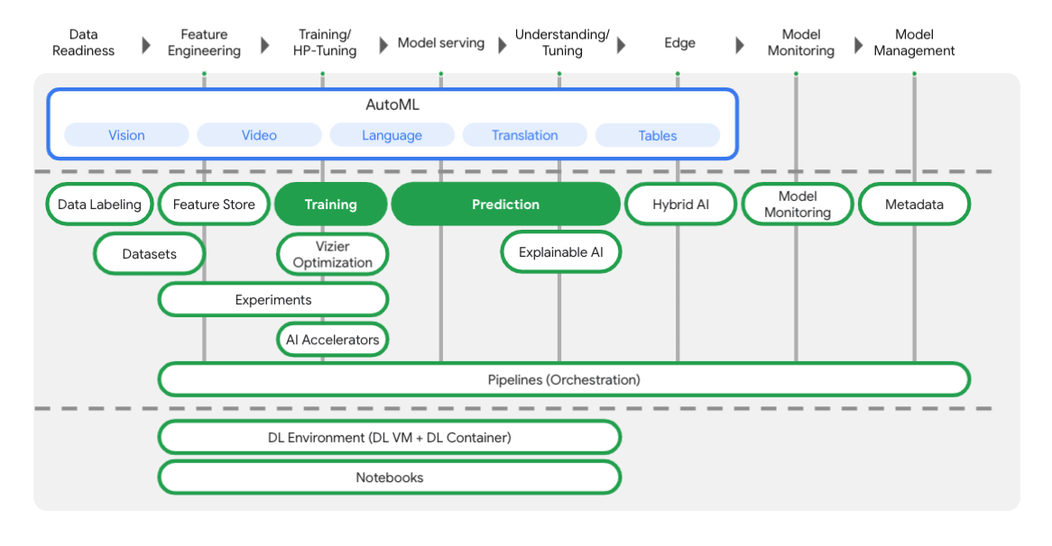
次の図に示すように、Vertex には ML ワークフローの各段階をサポートするさまざまなツールが用意されています。以下でハイライト表示されている Vertex Training と Prediction の使用に焦点を当てます。
3. 環境をセットアップする
セルフペース型の環境設定
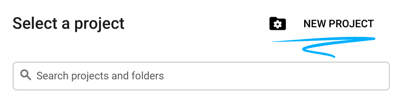
Cloud コンソールにログインして、新しいプロジェクトを作成するか、既存のプロジェクトを再利用します(Gmail アカウントも Google Workspace アカウントもまだお持ちでない場合は、アカウントを作成してください)。

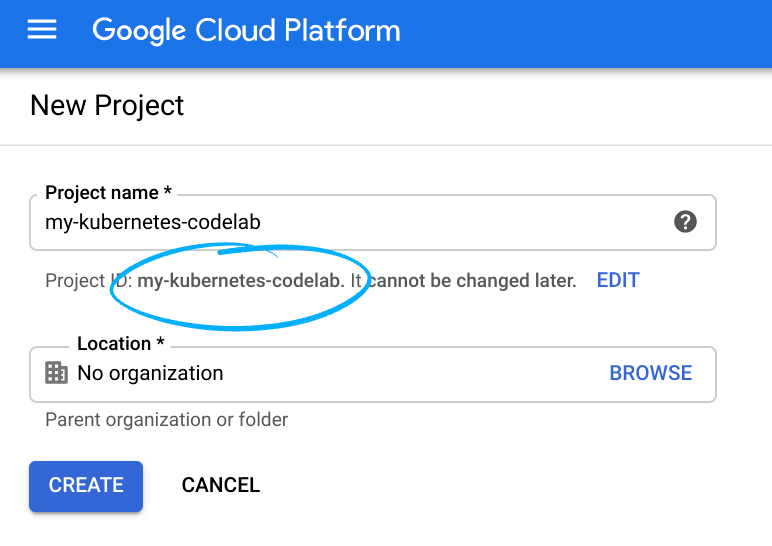
プロジェクト ID を忘れないようにしてください。プロジェクト ID はすべての Google Cloud プロジェクトを通じて一意の名前にする必要があります(上記の名前はすでに使用されているので使用できません)。
次に、Google Cloud リソースを使用するために、Cloud Console で課金を有効にする必要があります。
このコードラボを実行しても、費用はほとんどかからないはずです。このチュートリアル以外で請求が発生しないように、リソースのシャットダウン方法を説明する「クリーンアップ」セクションの手順に従うようにしてください。Google Cloud の新規ユーザーは、300 米ドル分の無料トライアル プログラムをご利用いただけます。
ステップ 1: Cloud Shell を起動する
このラボでは、Cloud Shell セッションで作業します。Cloud Shell は、Google のクラウド内で実行されている仮想マシンによってホストされたコマンド インタープリタです。このセクションは、パソコンでもローカルで簡単に実行できますが、Cloud Shell を使用することで、誰もが一貫した環境での再現可能な操作性を利用できるようになります。本ラボの後、このセクションをパソコン上で再度実行してみてください。
Cloud Shell をアクティブにする
Cloud コンソールの右上にある次のボタンをクリックして、Cloud Shell をアクティブにします。

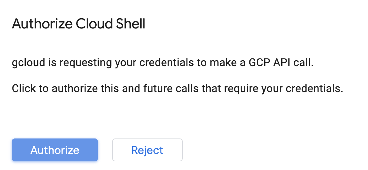
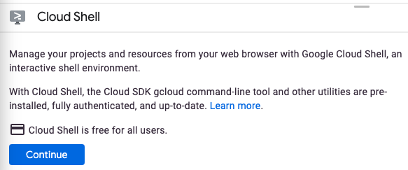
Cloud Shell を初めて起動した場合は、その内容を説明する画面が(スクロールしなければ見えない位置に)表示されます。その場合は、[続行] をクリックしてください(以後表示されなくなります)。この中間画面は次のようになります。
すぐにプロビジョニングが実行され、Cloud Shell に接続されます。
この仮想マシンには、必要な開発ツールがすべて用意されています。仮想マシンは Google Cloud で稼働し、永続的なホーム ディレクトリが 5 GB 用意されているため、ネットワークのパフォーマンスと認証が大幅に向上しています。このコードラボでの作業のほとんどは、ブラウザまたは Chromebook から実行できます。
Cloud Shell に接続すると、すでに認証は完了しており、プロジェクトに各自のプロジェクト ID が設定されていることがわかります。
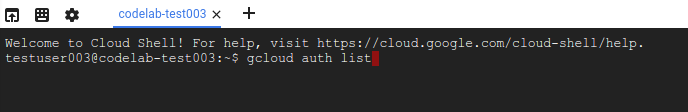
Cloud Shell で次のコマンドを実行して、認証されたことを確認します。
gcloud auth list
コマンド出力
 Credentialed Accounts
ACTIVE  ACCOUNT
*       <my_account>@<my_domain.com>

To set the active account, run:
    $ gcloud config set account `ACCOUNT`
Cloud Shell で次のコマンドを実行して、gcloud コマンドがプロジェクトを認識していることを確認します。
gcloud config list project
コマンド出力
[core]
project = <PROJECT_ID>
上記のようになっていない場合は、次のコマンドで設定できます。
gcloud config set project <PROJECT_ID>
コマンド出力
Updated property [core/project].
Cloud Shell には、現在のクラウド プロジェクトの名前が格納されている GOOGLE_CLOUD_PROJECT など、いくつかの環境変数があります。本ラボではさまざまな場所でこれを使用します。次を実行すると確認できます。
echo $GOOGLE_CLOUD_PROJECT
ステップ 2: API を有効にする
これらのサービスがどんな場面で(なぜ)必要になるのかは、後の手順でわかります。とりあえず、次のコマンドを実行して Compute Engine、Container Registry、Vertex AI の各サービスへのアクセス権をプロジェクトに付与します。
gcloud services enable compute.googleapis.com         \
                       containerregistry.googleapis.com  \
                       aiplatform.googleapis.com
成功すると次のようなメッセージが表示されます。
Operation "operations/acf.cc11852d-40af-47ad-9d59-477a12847c9e" finished successfully.
ステップ 3: Cloud Storage バケットを作成する
Vertex AI でトレーニング ジョブを実行するには、保存対象のモデルアセットを格納するストレージ バケットが必要です。Cloud Shell で次のコマンドを実行して、バケットを作成します。
BUCKET_NAME=gs://$GOOGLE_CLOUD_PROJECT-bucket
gsutil mb -l us-central1 $BUCKET_NAME
ステップ 4: Python 3 のエイリアスを作成する
このラボのコードでは Python 3 を使用します。このラボで作成するスクリプトを実行するときに Python 3 を使用するには、Cloud Shell で次のコマンドを実行してエイリアスを作成します。
alias python=python3
このラボでトレーニングして提供するモデルは、TensorFlow ドキュメントのこのチュートリアルに基づいています。このチュートリアルでは、Kaggle の Auto MPG データセットを使用して、自動車の燃料効率を予測します。
4. トレーニング コードをコンテナ化する
このトレーニング ジョブを Vertex に送信しましょう。トレーニング コードを Docker コンテナに格納して、このコンテナを Google Container Registry に push します。この方法を使用すると、どのフレームワークで構築されたモデルでもトレーニングできます。
ステップ 1: ファイルを設定する
まず、Cloud Shell のターミナルで次のコマンドを実行して、Docker コンテナに必要なファイルを作成します。
mkdir mpg
cd mpg
touch Dockerfile
mkdir trainer
touch trainer/train.py
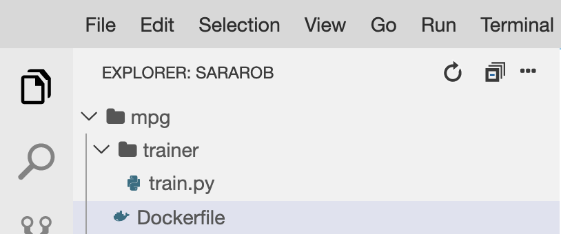
mpg/ ディレクトリは次のようになります。
+ Dockerfile
+ trainer/
    + train.py
これらのファイルを表示、編集するには、Cloud Shell の組み込みコードエディタを使用します。Cloud Shell の右上にあるメニューバーのボタンをクリックすると、エディタとターミナルを切り替えることができます。

ステップ 2: Dockerfile を作成する
コードをコンテナ化するには、まず Dockerfile を作成します。Dockerfile には、イメージの実行に必要なすべてのコマンドを含めます。使用しているすべてのライブラリがインストールされ、トレーニング コードのエントリ ポイントが設定されます。
Cloud Shell ファイル エディタで、mpg/ ディレクトリを開き、ダブルクリックして Dockerfile を開きます。
次に、以下の内容をこのファイルにコピーします。
FROM gcr.io/deeplearning-platform-release/tf2-cpu.2-3
WORKDIR /

# Copies the trainer code to the docker image.
COPY trainer /trainer

# Sets up the entry point to invoke the trainer.
ENTRYPOINT ["python", "-m", "trainer.train"]
この Dockerfile は、Deep Learning Containers TensorFlow Enterprise 2.3 Docker イメージを使用します。Google Cloud の Deep Learning Containers には一般的な ML およびデータ サイエンスのフレームワークが数多くプリインストールされています。使用しているものには、TF Enterprise 2.3、Pandas、Scikit-learn などが含まれます。この Dockerfile は、該当するイメージをダウンロードした後、トレーニング コードのエントリ ポイントを設定します。このコードは次のステップで追加します。
ステップ 3: モデルのトレーニング コードを追加する
Cloud Shell エディタで、train.py ファイルを開き、次のコードをコピーします(これは TensorFlow ドキュメントのチュートリアルから引用しています)。
# This will be replaced with your bucket name after running the `sed` command in the tutorial
BUCKET = "BUCKET_NAME"

import numpy as np
import pandas as pd
import pathlib
import tensorflow as tf

from tensorflow import keras
from tensorflow.keras import layers

print(tf.__version__)

"""## The Auto MPG dataset

The dataset is available from the [UCI Machine Learning Repository](https://archive.ics.uci.edu/ml/).

### Get the data
First download the dataset.
"""

"""Import it using pandas"""

dataset_path = "https://storage.googleapis.com/io-vertex-codelab/auto-mpg.csv"
dataset = pd.read_csv(dataset_path, na_values = "?")

dataset.tail()

"""### Clean the data

The dataset contains a few unknown values.
"""

dataset.isna().sum()

"""To keep this initial tutorial simple drop those rows."""

dataset = dataset.dropna()

"""The `"origin"` column is really categorical, not numeric. So convert that to a one-hot:"""

dataset['origin'] = dataset['origin'].map({1: 'USA', 2: 'Europe', 3: 'Japan'})

dataset = pd.get_dummies(dataset, prefix='', prefix_sep='')
dataset.tail()

"""### Split the data into train and test

Now split the dataset into a training set and a test set.

We will use the test set in the final evaluation of our model.
"""

train_dataset = dataset.sample(frac=0.8,random_state=0)
test_dataset = dataset.drop(train_dataset.index)

"""### Inspect the data

Have a quick look at the joint distribution of a few pairs of columns from the training set.

Also look at the overall statistics:
"""

train_stats = train_dataset.describe()
train_stats.pop("mpg")
train_stats = train_stats.transpose()
train_stats

"""### Split features from labels

Separate the target value, or "label", from the features. This label is the value that you will train the model to predict.
"""

train_labels = train_dataset.pop('mpg')
test_labels = test_dataset.pop('mpg')

"""### Normalize the data

Look again at the `train_stats` block above and note how different the ranges of each feature are.

It is good practice to normalize features that use different scales and ranges. Although the model *might* converge without feature normalization, it makes training more difficult, and it makes the resulting model dependent on the choice of units used in the input.

Note: Although we intentionally generate these statistics from only the training dataset, these statistics will also be used to normalize the test dataset. We need to do that to project the test dataset into the same distribution that the model has been trained on.
"""

def norm(x):
  return (x - train_stats['mean']) / train_stats['std']
normed_train_data = norm(train_dataset)
normed_test_data = norm(test_dataset)

"""This normalized data is what we will use to train the model.

Caution: The statistics used to normalize the inputs here (mean and standard deviation) need to be applied to any other data that is fed to the model, along with the one-hot encoding that we did earlier.  That includes the test set as well as live data when the model is used in production.

## The model

### Build the model

Let's build our model. Here, we'll use a `Sequential` model with two densely connected hidden layers, and an output layer that returns a single, continuous value. The model building steps are wrapped in a function, `build_model`, since we'll create a second model, later on.
"""

def build_model():
  model = keras.Sequential([
    layers.Dense(64, activation='relu', input_shape=[len(train_dataset.keys())]),
    layers.Dense(64, activation='relu'),
    layers.Dense(1)
  ])

  optimizer = tf.keras.optimizers.RMSprop(0.001)

  model.compile(loss='mse',
                optimizer=optimizer,
                metrics=['mae', 'mse'])
  return model

model = build_model()

"""### Inspect the model

Use the `.summary` method to print a simple description of the model
"""

model.summary()

"""Now try out the model. Take a batch of `10` examples from the training data and call `model.predict` on it.

It seems to be working, and it produces a result of the expected shape and type.

### Train the model

Train the model for 1000 epochs, and record the training and validation accuracy in the `history` object.

Visualize the model's training progress using the stats stored in the `history` object.

This graph shows little improvement, or even degradation in the validation error after about 100 epochs. Let's update the `model.fit` call to automatically stop training when the validation score doesn't improve. We'll use an *EarlyStopping callback* that tests a training condition for  every epoch. If a set amount of epochs elapses without showing improvement, then automatically stop the training.

You can learn more about this callback [here](https://www.tensorflow.org/api_docs/python/tf/keras/callbacks/EarlyStopping).
"""

model = build_model()

EPOCHS = 1000

# The patience parameter is the amount of epochs to check for improvement
early_stop = keras.callbacks.EarlyStopping(monitor='val_loss', patience=10)

early_history = model.fit(normed_train_data, train_labels,
                    epochs=EPOCHS, validation_split = 0.2,
                    callbacks=[early_stop])


# Export model and save to GCS
model.save(BUCKET + '/mpg/model')
上記のコードを mpg/trainer/train.py ファイルにコピーしたら、Cloud Shell のターミナルに戻り、次のコマンドを実行して、独自のバケット名をファイルに追加します。
sed -i "s|BUCKET_NAME|$BUCKET_NAME|g" trainer/train.py
ステップ 4: コンテナをローカルでビルドしてテストする
ターミナルから次のコマンドを実行して、Google Container Registry 内のコンテナ イメージの URI を示す変数を定義します。
IMAGE_URI="gcr.io/$GOOGLE_CLOUD_PROJECT/mpg:v1"
続いて、mpg ディレクトリのルートで次のように実行してコンテナをビルドします。
docker build ./ -t $IMAGE_URI
コンテナをビルドしたら、Google Container Registry に push します。
docker push $IMAGE_URI
イメージが Container Registry に push されたことを確認するには、コンソールの Container Registry セクションに移動すると、次のような内容が表示されます。
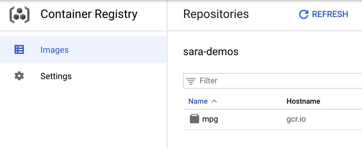
コンテナを Container Registry に push したら、カスタムモデルのトレーニング ジョブをいつでも開始できます。
5. Vertex AI でトレーニング ジョブを実行する
Vertex では、次の 2 つの方法でモデルをトレーニングできます。
- AutoML: 最小限の労力と ML の専門知識で高品質なモデルをトレーニングする
- カスタム トレーニング: Google Cloud のビルド済みコンテナまたは独自のコンテナのいずれかを使用して、クラウド内でカスタム トレーニング アプリケーションを実行します。
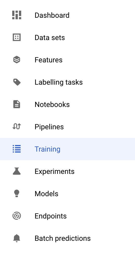
このラボでは、Google Container Registry 上の独自のカスタム コンテナを使用してカスタム トレーニングを行います。まず、Cloud コンソールの Vertex で [トレーニング] セクションに移動します。
ステップ 1: トレーニング ジョブを開始する
[作成] をクリックして、トレーニング ジョブとデプロイされたモデルのパラメータを入力します。
- [Dataset] で [マネージド データセットなし] を選択します。
- トレーニング方法として [カスタム トレーニング(上級者向け)] を選択し、[続行] をクリックします。
- [モデル名] に「
mpg」と入力します(または任意のモデル名を入力します)。 - [続行] をクリックする
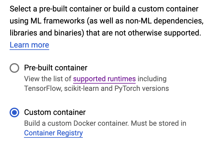
コンテナの設定ステップで、[カスタム コンテナ] を選択します。
最初のボックス(コンテナ イメージ)で、[参照] をクリックして、Container Registry に push したコンテナを見つけます。次のようになります。
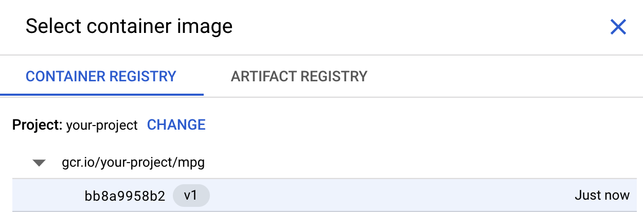
その他のフィールドは空白のままにして、[続行] をクリックします。
このチュートリアルではハイパーパラメータ チューニングを使用しないため、[ハイパーパラメータ チューニングを有効にする] ボックスのチェックをオフのままにして、[続行] をクリックします。
[コンピューティングと料金] で、選択されているリージョンはそのままにしておき、マシンタイプとして [n1-standard-4] を選択します。
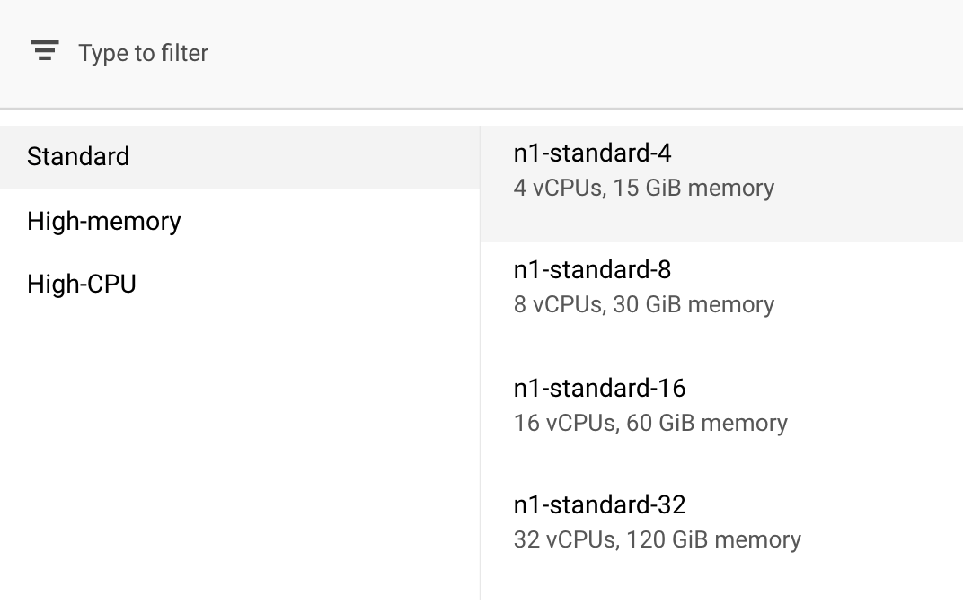
このデモのモデルは短時間でトレーニングが完了するため、小さめのマシンタイプを使用しています。
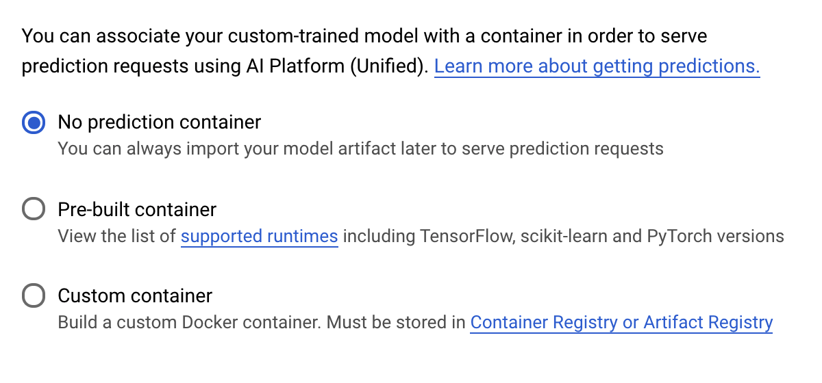
[予測コンテナ] ステップで、[予測コンテナなし] を選択します。
6. モデル エンドポイントをデプロイする
このステップでは、トレーニング済みモデルのエンドポイントを作成します。これを使用して、Vertex AI API 経由でモデルの予測を取得できます。このため、エクスポートされたトレーニング済みモデル アセットのバージョンを一般公開の GCS バケットで利用できるようにしました。
組織では、モデルの構築を担当するチームまたは個人と、モデルのデプロイを担当する別のチームが存在するのが一般的です。ここで説明する手順では、すでにトレーニング済みのモデルを取得して予測用にデプロイする方法について説明します。
ここでは、Vertex AI SDK を使用してモデルを作成し、エンドポイントにデプロイして、予測を取得します。
ステップ 1: Vertex SDK をインストールする
Cloud Shell ターミナルから、次のコマンドを実行して Vertex AI SDK をインストールします。
pip3 install google-cloud-aiplatform --upgrade --user
この SDK を使用して、Vertex のさまざまな部分を操作できます。
ステップ 2: モデルを作成してエンドポイントをデプロイする
次に、Python ファイルを作成し、SDK を使用してモデルリソースを作成してエンドポイントにデプロイします。Cloud Shell のファイル エディタで、[File]、[New File] の順に選択します。
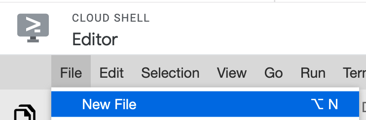
ファイル名を deploy.py とします。このファイルをエディタで開き、次のコードをコピーします。
from google.cloud import aiplatform

# Create a model resource from public model assets
model = aiplatform.Model.upload(
    display_name="mpg-imported",
    artifact_uri="gs://io-vertex-codelab/mpg-model/",
    serving_container_image_uri="gcr.io/cloud-aiplatform/prediction/tf2-cpu.2-3:latest"
)

# Deploy the above model to an endpoint
endpoint = model.deploy(
    machine_type="n1-standard-4"
)
次に、Cloud Shell のターミナルに戻り、cd でルート ディレクトリに戻り、作成した Python スクリプトを実行します。
cd ..
python3 deploy.py | tee deploy-output.txt
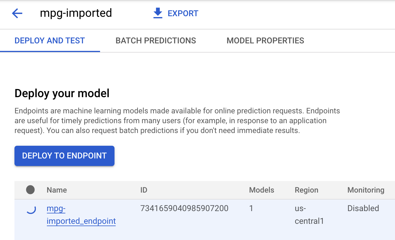
リソースの作成中に、ターミナルに更新が記録されます。このコマンドの実行には 10 ~ 15 分かかります。正しく動作していることを確認するには、Vertex AI のコンソールの [モデル] セクションに移動します。
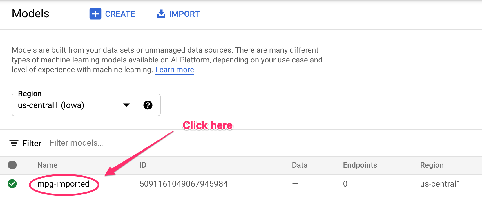
[mgp-imported] をクリックすると、そのモデルのエンドポイントが作成されていることがわかります。
Cloud Shell ターミナルには、エンドポイントのデプロイが完了すると、次のようなログが表示されます。
Endpoint model deployed. Resource name: projects/your-project-id/locations/us-central1/endpoints/your-endpoint-id
これは、次のステップでデプロイされたエンドポイントの予測を取得するために使用します。
ステップ 3: デプロイされたエンドポイントで予測を取得する
Cloud Shell エディタで、predict.py という名前の新しいファイルを作成します。
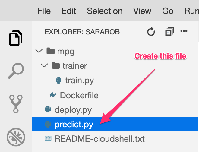
predict.py を開き、次のコードを貼り付けます。
from google.cloud import aiplatform

endpoint = aiplatform.Endpoint(
    endpoint_name="ENDPOINT_STRING"
)

# A test example we'll send to our model for prediction
test_mpg = [1.4838871833555929,
 1.8659883497083019,
 2.234620276849616,
 1.0187816540094903,
 -2.530890710602246,
 -1.6046416850441676,
 -0.4651483719733302,
 -0.4952254087173721,
 0.7746763768735953]

response = endpoint.predict([test_mpg])

print('API response: ', response)

print('Predicted MPG: ', response.predictions[0][0])
次に、ターミナルに戻り、次のコマンドを入力して、予測ファイルの ENDPOINT_STRING を独自のエンドポイントに置き換えます。
ENDPOINT=$(cat deploy-output.txt | sed -nre 's:.*Resource name\: (.*):\1:p' | tail -1)
sed -i "s|ENDPOINT_STRING|$ENDPOINT|g" predict.py
次に、predict.py ファイルを実行して、デプロイされたモデル エンドポイントから予測を取得します。
python3 predict.py
API のレスポンスがログに記録され、テスト予測の予測燃料効率が表示されます。
お疲れさまでした
Vertex AI を使って次のことを行う方法を学びました。
- カスタム コンテナにトレーニング コードを提供してモデルをトレーニングする。ここでは例として TensorFlow モデルを使用しましたが、カスタム コンテナを使って任意のフレームワークで構築されたモデルをトレーニングすることができます。
- トレーニングに使用したのと同じワークフローの一環として、ビルド済みコンテナを使用して TensorFlow モデルをデプロイする。
- モデルのエンドポイントを作成し、予測を生成する。
Vertex AI のさまざまな機能の詳細については、ドキュメントをご覧ください。ステップ 5 で開始したトレーニング ジョブの結果を確認するには、Vertex コンソールのトレーニング セクションに移動します。
7. クリーンアップ
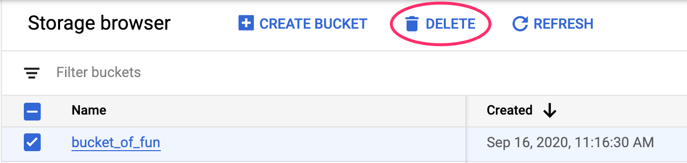
デプロイしたエンドポイントを削除するには、Vertex コンソールの [エンドポイント] セクションに移動し、削除アイコンをクリックします。

ストレージ バケットを削除するには、Cloud コンソールのナビゲーション メニューで [ストレージ] に移動してバケットを選択し、[削除] をクリックします。